Warning: package 'dslabs' was built under R version 4.5.2
# only run the next command interactively, not in a script# help(gapminder) # get an overview of data structurestr(gapminder)
'data.frame':   10545 obs. of  9 variables:
 $ country         : Factor w/ 185 levels "Albania","Algeria",..: 1 2 3 4 5 6 7 8 9 10 ...
 $ year            : int  1960 1960 1960 1960 1960 1960 1960 1960 1960 1960 ...
 $ infant_mortality: num  115.4 148.2 208 NA 59.9 ...
 $ life_expectancy : num  62.9 47.5 36 63 65.4 ...
 $ fertility       : num  6.19 7.65 7.32 4.43 3.11 4.55 4.82 3.45 2.7 5.57 ...
 $ population      : num  1636054 11124892 5270844 54681 20619075 ...
 $ gdp             : num  NA 1.38e+10 NA NA 1.08e+11 ...
 $ continent       : Factor w/ 5 levels "Africa","Americas",..: 4 1 1 2 2 3 2 5 4 3 ...
 $ region          : Factor w/ 22 levels "Australia and New Zealand",..: 19 11 10 2 15 21 2 1 22 21 ...
# get a summary of datasummary(gapminder)
                country           year      infant_mortality life_expectancy
 Albania            :   57   Min.   :1960   Min.   :  1.50   Min.   :13.20
 Algeria            :   57   1st Qu.:1974   1st Qu.: 16.00   1st Qu.:57.50
 Angola             :   57   Median :1988   Median : 41.50   Median :67.54
 Antigua and Barbuda:   57   Mean   :1988   Mean   : 55.31   Mean   :64.81
 Argentina          :   57   3rd Qu.:2002   3rd Qu.: 85.10   3rd Qu.:73.00
 Armenia            :   57   Max.   :2016   Max.   :276.90   Max.   :83.90
 (Other)            :10203                  NA's   :1453
   fertility       population             gdp               continent
 Min.   :0.840   Min.   :3.124e+04   Min.   :4.040e+07   Africa  :2907
 1st Qu.:2.200   1st Qu.:1.333e+06   1st Qu.:1.846e+09   Americas:2052
 Median :3.750   Median :5.009e+06   Median :7.794e+09   Asia    :2679
 Mean   :4.084   Mean   :2.701e+07   Mean   :1.480e+11   Europe  :2223
 3rd Qu.:6.000   3rd Qu.:1.523e+07   3rd Qu.:5.540e+10   Oceania : 684
 Max.   :9.220   Max.   :1.376e+09   Max.   :1.174e+13
 NA's   :187     NA's   :185         NA's   :2972
             region
 Western Asia   :1026
 Eastern Africa : 912
 Western Africa : 912
 Caribbean      : 741
 South America  : 684
 Southern Europe: 684
 (Other)        :5586
# determine the type of object gapminder isclass(gapminder)
[1] "data.frame"
africandata <-subset(gapminder, continent %in%"Africa") #subsetting data for african countries# get an overview of data structurestr(africandata)
'data.frame':   2907 obs. of  9 variables:
 $ country         : Factor w/ 185 levels "Albania","Algeria",..: 2 3 18 22 26 27 29 31 32 33 ...
 $ year            : int  1960 1960 1960 1960 1960 1960 1960 1960 1960 1960 ...
 $ infant_mortality: num  148 208 187 116 161 ...
 $ life_expectancy : num  47.5 36 38.3 50.3 35.2 ...
 $ fertility       : num  7.65 7.32 6.28 6.62 6.29 6.95 5.65 6.89 5.84 6.25 ...
 $ population      : num  11124892 5270844 2431620 524029 4829291 ...
 $ gdp             : num  1.38e+10 NA 6.22e+08 1.24e+08 5.97e+08 ...
 $ continent       : Factor w/ 5 levels "Africa","Americas",..: 1 1 1 1 1 1 1 1 1 1 ...
 $ region          : Factor w/ 22 levels "Australia and New Zealand",..: 11 10 20 17 20 5 10 20 10 10 ...
# get a summary of datasummary(africandata)
         country          year      infant_mortality life_expectancy
 Algeria     :  57   Min.   :1960   Min.   : 11.40   Min.   :13.20
 Angola      :  57   1st Qu.:1974   1st Qu.: 62.20   1st Qu.:48.23
 Benin       :  57   Median :1988   Median : 93.40   Median :53.98
 Botswana    :  57   Mean   :1988   Mean   : 95.12   Mean   :54.38
 Burkina Faso:  57   3rd Qu.:2002   3rd Qu.:124.70   3rd Qu.:60.10
 Burundi     :  57   Max.   :2016   Max.   :237.40   Max.   :77.60
 (Other)     :2565                  NA's   :226
   fertility       population             gdp               continent
 Min.   :1.500   Min.   :    41538   Min.   :4.659e+07   Africa  :2907
 1st Qu.:5.160   1st Qu.:  1605232   1st Qu.:8.373e+08   Americas:   0
 Median :6.160   Median :  5570982   Median :2.448e+09   Asia    :   0
 Mean   :5.851   Mean   : 12235961   Mean   :9.346e+09   Europe  :   0
 3rd Qu.:6.860   3rd Qu.: 13888152   3rd Qu.:6.552e+09   Oceania :   0
 Max.   :8.450   Max.   :182201962   Max.   :1.935e+11
 NA's   :51      NA's   :51          NA's   :637
                       region
 Eastern Africa           :912
 Western Africa           :912
 Middle Africa            :456
 Northern Africa          :342
 Southern Africa          :285
 Australia and New Zealand:  0
 (Other)                  :  0
# determine the type of object
class(africandata)
[1] "data.frame"
infant_mortality_data <-data.frame(africandata$infant_mortality, africandata$life_expectancy) #making a dataframe for infant mortalitypopulation_data <-data.frame(africandata$population, africandata$life_expectancy) #making a dataframe for infant mortality
# get an overview of data structurestr(infant_mortality_data)
'data.frame':   2907 obs. of  2 variables:
 $ africandata.infant_mortality: num  148 208 187 116 161 ...
 $ africandata.life_expectancy : num  47.5 36 38.3 50.3 35.2 ...
# get a summary of datasummary(infant_mortality_data)
 africandata.infant_mortality africandata.life_expectancy
 Min.   : 11.40               Min.   :13.20
 1st Qu.: 62.20               1st Qu.:48.23
 Median : 93.40               Median :53.98
 Mean   : 95.12               Mean   :54.38
 3rd Qu.:124.70               3rd Qu.:60.10
 Max.   :237.40               Max.   :77.60
 NA's   :226
# get an overview of data structurestr(population_data)
'data.frame':   2907 obs. of  2 variables:
 $ africandata.population     : num  11124892 5270844 2431620 524029 4829291 ...
 $ africandata.life_expectancy: num  47.5 36 38.3 50.3 35.2 ...
# get a summary of datasummary(population_data)
 africandata.population africandata.life_expectancy
 Min.   :    41538      Min.   :13.20
 1st Qu.:  1605232      1st Qu.:48.23
 Median :  5570982      Median :53.98
 Mean   : 12235961      Mean   :54.38
 3rd Qu.: 13888152      3rd Qu.:60.10
 Max.   :182201962      Max.   :77.60
 NA's   :51
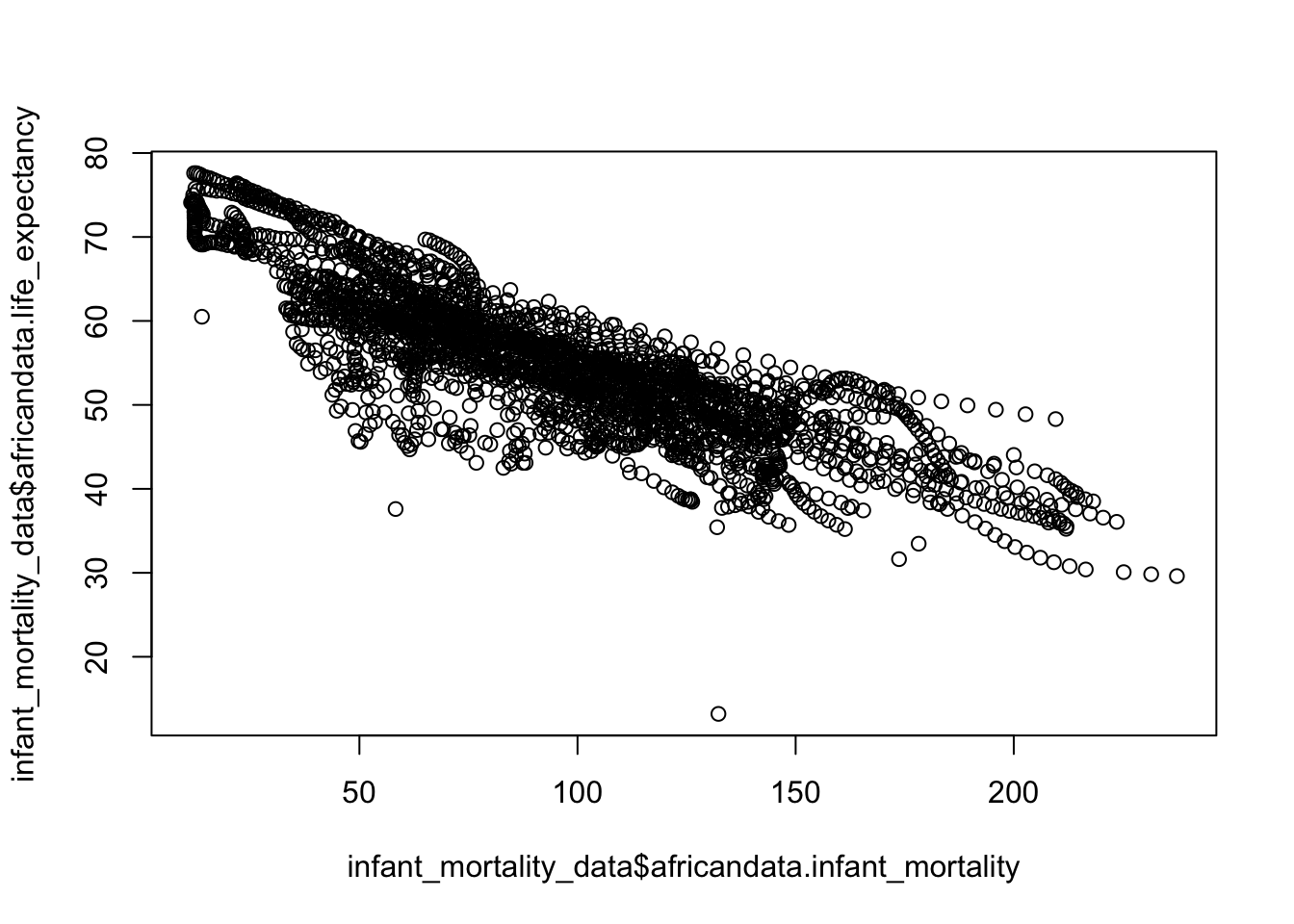
#ploting infant mortality vs life expectancyplot(infant_mortality_data$africandata.infant_mortality, infant_mortality_data$africandata.life_expectancy)
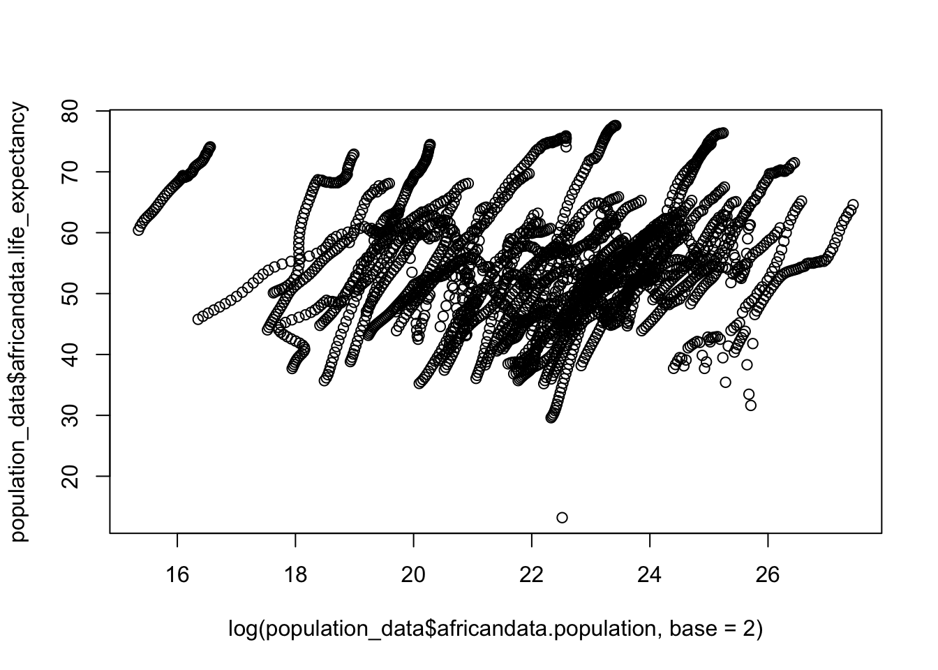
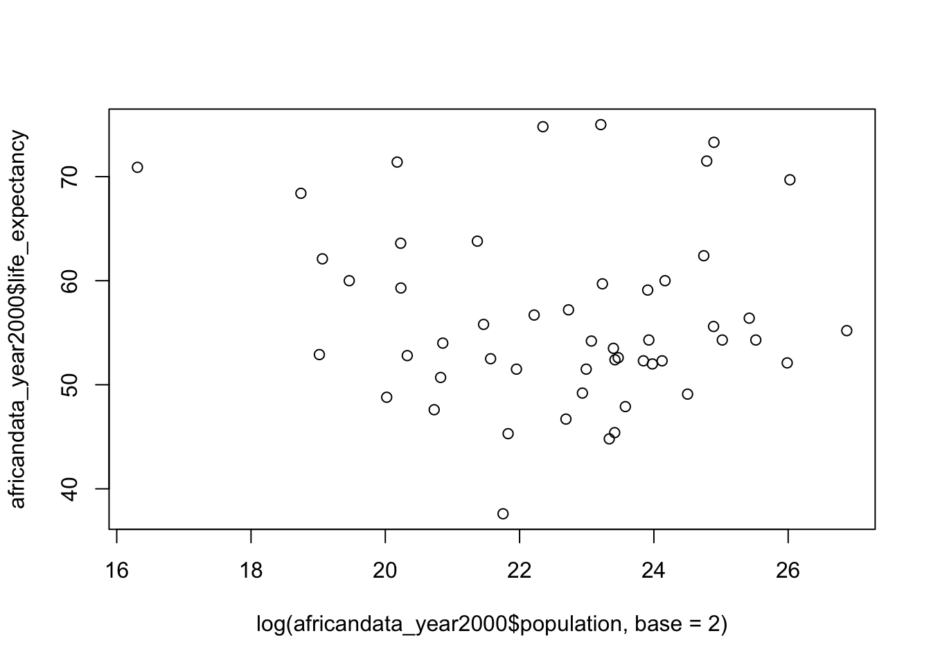
#ploting population vs life expectancyplot(log(population_data$africandata.population, base =2), population_data$africandata.life_expectancy)
# In both plots, streak patterns occur because each country contributes multiple times across different years and they tend to grow.
africandata_year2000 <-subset(africandata, year %in%2000)# get an overview of data structurestr(africandata_year2000)
'data.frame':   51 obs. of  9 variables:
 $ country         : Factor w/ 185 levels "Albania","Algeria",..: 2 3 18 22 26 27 29 31 32 33 ...
 $ year            : int  2000 2000 2000 2000 2000 2000 2000 2000 2000 2000 ...
 $ infant_mortality: num  33.9 128.3 89.3 52.4 96.2 ...
 $ life_expectancy : num  73.3 52.3 57.2 47.6 52.6 46.7 54.3 68.4 45.3 51.5 ...
 $ fertility       : num  2.51 6.84 5.98 3.41 6.59 7.06 5.62 3.7 5.45 7.35 ...
 $ population      : num  31183658 15058638 6949366 1736579 11607944 ...
 $ gdp             : num  5.48e+10 9.13e+09 2.25e+09 5.63e+09 2.61e+09 ...
 $ continent       : Factor w/ 5 levels "Africa","Americas",..: 1 1 1 1 1 1 1 1 1 1 ...
 $ region          : Factor w/ 22 levels "Australia and New Zealand",..: 11 10 20 17 20 5 10 20 10 10 ...
# get a summary of datasummary(africandata_year2000)
         country        year      infant_mortality life_expectancy
 Algeria     : 1   Min.   :2000   Min.   : 12.30   Min.   :37.60
 Angola      : 1   1st Qu.:2000   1st Qu.: 60.80   1st Qu.:51.75
 Benin       : 1   Median :2000   Median : 80.30   Median :54.30
 Botswana    : 1   Mean   :2000   Mean   : 78.93   Mean   :56.36
 Burkina Faso: 1   3rd Qu.:2000   3rd Qu.:103.30   3rd Qu.:60.00
 Burundi     : 1   Max.   :2000   Max.   :143.30   Max.   :75.00
 (Other)     :45
   fertility       population             gdp               continent
 Min.   :1.990   Min.   :    81154   Min.   :2.019e+08   Africa  :51
 1st Qu.:4.150   1st Qu.:  2304687   1st Qu.:1.274e+09   Americas: 0
 Median :5.550   Median :  8799165   Median :3.238e+09   Asia    : 0
 Mean   :5.156   Mean   : 15659800   Mean   :1.155e+10   Europe  : 0
 3rd Qu.:5.960   3rd Qu.: 17391242   3rd Qu.:8.654e+09   Oceania : 0
 Max.   :7.730   Max.   :122876723   Max.   :1.329e+11

                       region
 Eastern Africa           :16
 Western Africa           :16
 Middle Africa            : 8
 Northern Africa          : 6
 Southern Africa          : 5
 Australia and New Zealand: 0
 (Other)                  : 0
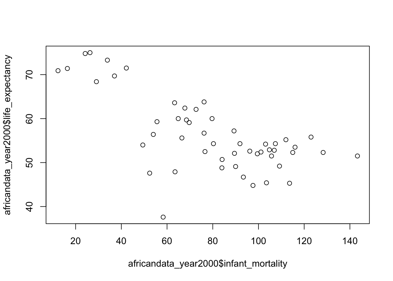
#replotting only year 2000plot(africandata_year2000$infant_mortality, africandata_year2000$life_expectancy)
plot(log(africandata_year2000$population, base =2), africandata_year2000$life_expectancy)
#lm base on year 2000fit1 <-lm(life_expectancy ~ infant_mortality, data = africandata_year2000)summary(fit1)
Call:
lm(formula = life_expectancy ~ infant_mortality, data = africandata_year2000)

Residuals:
     Min       1Q   Median       3Q      Max
-22.6651  -3.7087   0.9914   4.0408   8.6817

Coefficients:
                 Estimate Std. Error t value Pr(>|t|)
(Intercept)      71.29331    2.42611  29.386  < 2e-16 ***
infant_mortality -0.18916    0.02869  -6.594 2.83e-08 ***
---
Signif. codes:  0 '***' 0.001 '**' 0.01 '*' 0.05 '.' 0.1 ' ' 1

Residual standard error: 6.221 on 49 degrees of freedom
Multiple R-squared:  0.4701,    Adjusted R-squared:  0.4593
F-statistic: 43.48 on 1 and 49 DF,  p-value: 2.826e-08
fit2 <-lm(life_expectancy ~ population, data = africandata_year2000)summary(fit2)
Call:
lm(formula = life_expectancy ~ population, data = africandata_year2000)

Residuals:
    Min      1Q  Median      3Q     Max
-18.429  -4.602  -2.568   3.800  18.802

Coefficients:
             Estimate Std. Error t value Pr(>|t|)
(Intercept) 5.593e+01  1.468e+00  38.097   <2e-16 ***
population  2.756e-08  5.459e-08   0.505    0.616
---
Signif. codes:  0 '***' 0.001 '**' 0.01 '*' 0.05 '.' 0.1 ' ' 1

Residual standard error: 8.524 on 49 degrees of freedom
Multiple R-squared:  0.005176,  Adjusted R-squared:  -0.01513
F-statistic: 0.2549 on 1 and 49 DF,  p-value: 0.6159
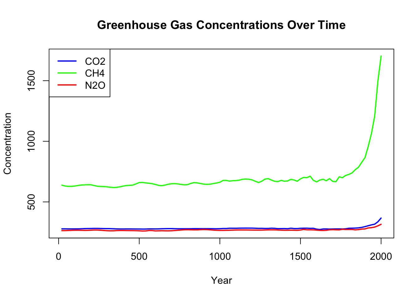
#This section contributed by Riley Herber.#More Data Exploration#Analysis of Concentrations of the three main greenhouse gases carbon dioxide, methane and nitrous oxide from 1-2000 CE.#summary(greenhouse_gases)data <- greenhouse_gases#creates a data.frame object for each gas including year and concentrationsCO2 <- greenhouse_gases[greenhouse_gases$gas =="CO2", ]CH4 <- greenhouse_gases[greenhouse_gases$gas =="CH4", ]N2O <- greenhouse_gases[greenhouse_gases$gas =="N2O", ]# set up an empty plot using all data to get axis limitsplot( greenhouse_gases$year, greenhouse_gases$concentration,type ="n", xlab ="Year",ylab ="Concentration",main ="Greenhouse Gas Concentrations Over Time")# add lines for each gaslines(CO2$year, CO2$concentration, col ="blue", lwd =2)lines(CH4$year, CH4$concentration, col ="green", lwd =2)lines(N2O$year, N2O$concentration, col ="red", lwd =2)# add legendlegend("topleft",legend =c("CO2", "CH4", "N2O"),col =c("blue", "green", "red"),lwd =2)
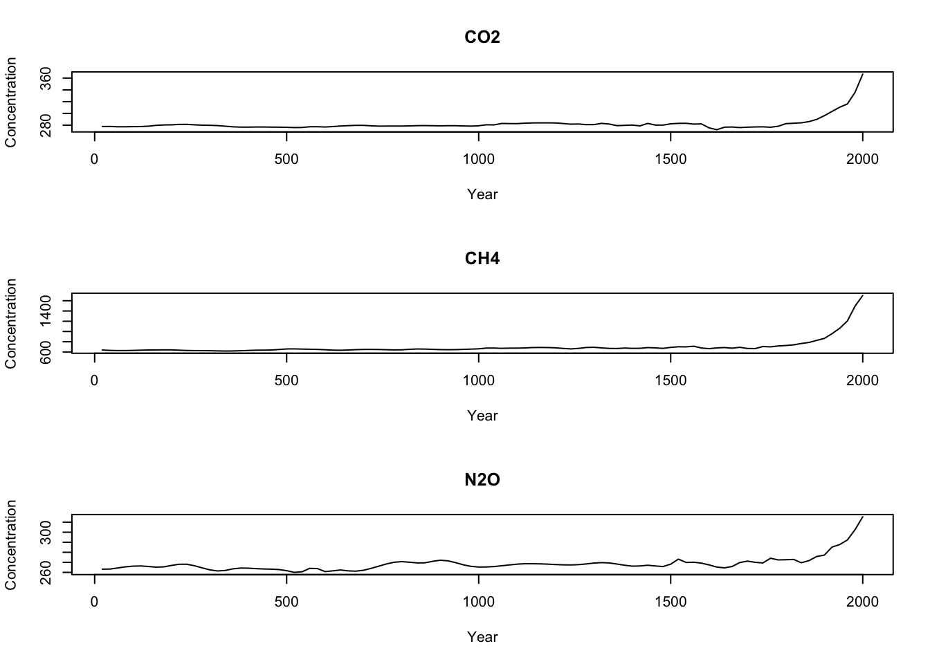
#ChatGPT was used to help me learn how to do multi-panel figure (code below)par(mfrow =c(3, 1)) # plot with 3 rows, 1 columnplot(CO2$year, CO2$concentration, type ="l",main ="CO2", xlab ="Year", ylab ="Concentration")plot(CH4$year, CH4$concentration, type ="l",main ="CH4", xlab ="Year", ylab ="Concentration")plot(N2O$year, N2O$concentration, type ="l",main ="N2O", xlab ="Year", ylab ="Concentration")
par(mfrow =c(1, 1)) # reset layoutfit3 <-lm(concentration ~ year * gas, data = greenhouse_gases)summary(fit3)
Call:
lm(formula = concentration ~ year * gas, data = greenhouse_gases)

Residuals:
    Min      1Q  Median      3Q     Max
-128.95   -6.83   -1.70    3.33  868.77

Coefficients:
              Estimate Std. Error t value Pr(>|t|)
(Intercept)  558.37400   15.44941  36.142  < 2e-16 ***
year           0.13813    0.01328  10.401  < 2e-16 ***
gasCO2      -285.06103   21.84876 -13.047  < 2e-16 ***
gasN2O      -297.83861   21.84876 -13.632  < 2e-16 ***
year:gasCO2   -0.12940    0.01878  -6.890 3.39e-11 ***
year:gasN2O   -0.13027    0.01878  -6.936 2.56e-11 ***
---
Signif. codes:  0 '***' 0.001 '**' 0.01 '*' 0.05 '.' 0.1 ' ' 1

Residual standard error: 76.67 on 294 degrees of freedom
Multiple R-squared:  0.879, Adjusted R-squared:  0.877
F-statistic: 427.2 on 5 and 294 DF,  p-value: < 2.2e-16
Analysis of greenhouse gas concentrations from 1–2000 CE revealed significant temporal trends that differed by gas type. Methane (CH4) exhibited a strong positive increase over time (CH4 slope = 0.138 per year and p < 0.001), whereas carbon dioxide (CO2) and nitrous oxide (N2O) had much lower baseline concentrations and minimal growth (CO2 adjusted slope = 0.009 per year; N2O adjusted slope = 0.008 per year; both p < 0.001). The interaction between year and gas was highly significant, indicating that the rate of increase varied across gases. Overall, the model explained 88% of the variance in concentrations (adjusted R-squared = 0.877), highlighting that CH4 has risen much more rapidly than CO2 or N2O over the past two millennia.