#Fitting exercise

# Loading data
library(here)

here() starts at C:/Users/marco/Documents/marcoreina-portafolio

data <- read.csv(here("fitting-exercise/", "Mavoglurant_A2121_nmpk.csv"))

str(data)

'data.frame':   2678 obs. of  17 variables:
 $ ID  : int  793 793 793 793 793 793 793 793 793 793 ...
 $ CMT : int  1 2 2 2 2 2 2 2 2 2 ...
 $ EVID: int  1 0 0 0 0 0 0 0 0 0 ...
 $ EVI2: int  1 0 0 0 0 0 0 0 0 0 ...
 $ MDV : int  1 0 0 0 0 0 0 0 0 0 ...
 $ DV  : num  0 491 605 556 310 237 147 101 72.4 52.6 ...
 $ LNDV: num  0 6.2 6.41 6.32 5.74 ...
 $ AMT : num  25 0 0 0 0 0 0 0 0 0 ...
 $ TIME: num  0 0.2 0.25 0.367 0.533 0.7 1.2 2.2 3.2 4.2 ...
 $ DOSE: num  25 25 25 25 25 25 25 25 25 25 ...
 $ OCC : int  1 1 1 1 1 1 1 1 1 1 ...
 $ RATE: int  75 0 0 0 0 0 0 0 0 0 ...
 $ AGE : int  42 42 42 42 42 42 42 42 42 42 ...
 $ SEX : int  1 1 1 1 1 1 1 1 1 1 ...
 $ RACE: int  2 2 2 2 2 2 2 2 2 2 ...
 $ WT  : num  94.3 94.3 94.3 94.3 94.3 94.3 94.3 94.3 94.3 94.3 ...
 $ HT  : num  1.77 1.77 1.77 1.77 1.77 ...

# Plotting DV ~ TIME
library(ggplot2)
ggplot(data, aes(y = DV, x = TIME)) + geom_point() + theme_bw()

ggplot(data, aes(y = DV, x = TIME, color = as.factor(DOSE))) + geom_point() + theme_bw()

ggplot(data, aes(y = DV, x = TIME, color = as.factor(DOSE))) + geom_point() + facet_wrap(~ DOSE) + theme_bw() + theme(strip.text = element_blank())

# Removing OCC = 2
data_occ1 <- subset(data, OCC == 1)

# Removing time = 0
data_timefilter <-  subset(data_occ1, !(TIME == 0))

# Data only with time zero
data_timezero <-  subset(data_occ1, (TIME == 0))

library(dplyr)

Attaching package: 'dplyr'

The following objects are masked from 'package:stats':

    filter, lag

The following objects are masked from 'package:base':

    intersect, setdiff, setequal, union

# Summarizing - ChatGPT used for this code
sum_dv <- data_occ1 %>%
  filter(TIME != 0) %>%
  group_by(ID) %>%
  summarize(Y = sum(DV, na.rm = TRUE))

# Merging datasets
merged_data <- left_join(data_timezero, sum_dv, by = "ID")

# "Last" data cleaning
data_clean <- data.frame(Y  = merged_data$Y,
                        DOSE = merged_data$DOSE,
                        AGE = merged_data$AGE,
                        SEX = as.factor(merged_data$SEX),
                        RACE = as.factor(merged_data$RACE),
                        WT = merged_data$WT,
                        HT = merged_data$HT)

library(readr)
write_csv(data_clean, here("fitting-exercise/", "data_clean.csv"))

# Plotting distributions for each one of the variables
hist(data_clean$Y) # Normally distirbuted, slight right skew

hist(data_clean$DOSE) # 3 doses used, will move to as.factor for certain plots

hist(data_clean$AGE) # few observation in 30-35 bin 

plot(data_clean$SEX) # sex 1 overrepresented

plot(data_clean$RACE) # Race 7 underrepresented

hist(data_clean$WT) # Normally distributed

hist(data_clean$HT) # Normally distributed

# First round of plots
ggplot(data_clean, aes(y = Y, x = as.factor(DOSE))) + geom_boxplot() + theme_bw() # Hihgher dose, higher Y

ggplot(data_clean, aes(y = Y, x = AGE)) + geom_point() + theme_bw() # No clear pattern observed

ggplot(data_clean, aes(y = Y, x = SEX)) + geom_boxplot() + theme_bw() # Similar distributuion of SEX 1 and 2

ggplot(data_clean, aes(y = Y, x = RACE)) + geom_boxplot() + theme_bw() #Similar distribution for RACE 1, 2, 7, and 88

ggplot(data_clean, aes(y = Y, x = WT)) + geom_point() + theme_bw() # No clear pattern observed

ggplot(data_clean, aes(y = Y, x = HT)) + geom_point() + theme_bw() # No clear pattern observed

# Second round of plots
ggplot(data_clean, aes(y = Y, x = as.factor(DOSE), levels =  SEX, fill = SEX)) + geom_boxplot() + theme_bw() # DOSE = 37.5 has wider distribution for SEX = 1

ggplot(data_clean, aes(y = Y, x = as.factor(DOSE), levels =  RACE, fill = RACE)) + geom_boxplot() + theme_bw() # DOSE = 37.5 has no representation of RACE = 7 and 88

ggplot(data_clean, aes(y = Y, x = WT, color = SEX)) + geom_point(size = 3) + theme_bw() + facet_wrap(~ SEX) + theme(strip.text = element_blank()) # SEX = 2 underrepresented as mentioned before, weight is less than SEX = 1

ggplot(data_clean, aes(y = Y, x = HT, color = RACE)) + geom_point(size = 3) + theme_bw() + facet_wrap(~ RACE) + theme(strip.text = element_blank()) # Only two observations of RACE = 7, very few observations of RACE = 88

ggplot(data_clean, aes(y = Y, x = WT, color = AGE, size = AGE)) + geom_point(alpha = 0.75) + theme_bw() # No clear pattern observed

ggplot(data_clean, aes(y = Y, x = HT, color = AGE, size = AGE)) + geom_point(alpha = 0.75) + theme_bw() # No clear pattern observed

library(tidymodels)

── Attaching packages ────────────────────────────────────── tidymodels 1.4.1 ──

✔ broom        1.0.12     ✔ rsample      1.3.2 
✔ dials        1.4.2      ✔ tailor       0.1.0 
✔ infer        1.1.0      ✔ tidyr        1.3.2 
✔ modeldata    1.5.1      ✔ tune         2.0.1 
✔ parsnip      1.4.1      ✔ workflows    1.3.0 
✔ purrr        1.2.1      ✔ workflowsets 1.1.1 
✔ recipes      1.3.1      ✔ yardstick    1.3.2 

── Conflicts ───────────────────────────────────────── tidymodels_conflicts() ──
✖ purrr::discard()  masks scales::discard()
✖ dplyr::filter()   masks stats::filter()
✖ dplyr::lag()      masks stats::lag()
✖ yardstick::spec() masks readr::spec()
✖ recipes::step()   masks stats::step()

library(dotwhisker)

#Loading engine for lm
linear_reg() %>% 
  set_engine("keras")

Linear Regression Model Specification (regression)

Computational engine: keras 

# Making first lm fit based on tidymodels, Y ~ DOSE
lm_mod1 <- linear_reg()

lm_fit1 <- 
  lm_mod1 %>% 
  fit(Y ~ DOSE, data = data_clean)

# Predictions: from ChatGPT
pred_lm1 <- predict(lm_fit1, data_clean) %>%
  bind_cols(data_clean)

# Metrics: from ChatGPT
metrics(pred_lm1, truth = Y, estimate = .pred)

# A tibble: 3 × 3
  .metric .estimator .estimate
  <chr>   <chr>          <dbl>
1 rmse    standard     666.   
2 rsq     standard       0.516
3 mae     standard     517.   

# Creating table of coefficients
tidy(lm_fit1)

# A tibble: 2 × 5
  term        estimate std.error statistic  p.value
  <chr>          <dbl>     <dbl>     <dbl>    <dbl>
1 (Intercept)    323.     199.        1.62 1.07e- 1
2 DOSE            58.2      5.19     11.2  2.69e-20

# Plotting first fit
tidy(lm_fit1) %>% 
  dwplot(dot_args = list(size = 2, color = "black"),
         whisker_args = list(color = "black"),
         vline = geom_vline(xintercept = 0, colour = "grey50", linetype = 2))

# Making second lm fit based on tidymodels, Y ~ DOSE + AGE + SEX + RACE + WT + HT
lm_mod2 <- linear_reg()

lm_fit2 <- 
  lm_mod2 %>% 
  fit(Y ~ DOSE + AGE + SEX + RACE + WT + HT, data = data_clean)

# Predictions: from ChatGPT
pred_lm2 <- predict(lm_fit2, data_clean) %>%
  bind_cols(data_clean)

# Metrics: from ChatGPT
metrics(pred_lm2, truth = Y, estimate = .pred)

# A tibble: 3 × 3
  .metric .estimator .estimate
  <chr>   <chr>          <dbl>
1 rmse    standard     591.   
2 rsq     standard       0.619
3 mae     standard     444.   

# Creating table of coefficients
tidy(lm_fit2)

# A tibble: 9 × 5
  term        estimate std.error statistic  p.value
  <chr>          <dbl>     <dbl>     <dbl>    <dbl>
1 (Intercept)  3387.     1835.       1.85  6.76e- 2
2 DOSE           59.9       4.88    12.3   2.05e-22
3 AGE             3.16      7.82     0.403 6.88e- 1
4 SEX2         -358.      217.      -1.65  1.02e- 1
5 RACE2         155.      129.       1.21  2.31e- 1
6 RACE7        -405.      448.      -0.904 3.68e- 1
7 RACE88        -53.5     245.      -0.219 8.27e- 1
8 WT            -23.0       6.40    -3.60  4.71e- 4
9 HT           -748.     1104.      -0.678 4.99e- 1

# Plotting second fit
tidy(lm_fit2) %>% 
  dwplot(dot_args = list(size = 2, color = "black"),
         whisker_args = list(color = "black"),
         vline = geom_vline(xintercept = 0, colour = "grey50", linetype = 2))

#Loading engine for glm
logistic_reg() %>% 
  set_engine("glm")

Logistic Regression Model Specification (classification)

Computational engine: glm 

# Making first glm fit based on tidymodels, Y ~ DOSE
log_mod1 <- logistic_reg() 

log_fit1 <- 
  log_mod1 %>% 
  fit(SEX ~ DOSE, data = data_clean)

# Predictions
pred_log1 <- predict(log_fit1, data_clean, type = "prob") %>%
  bind_cols(predict(log_fit1, data_clean)) %>%
  bind_cols(data_clean)

# Metrics
accuracy(pred_log1, truth = SEX, estimate = .pred_class)

# A tibble: 1 × 3
  .metric  .estimator .estimate
  <chr>    <chr>          <dbl>
1 accuracy binary         0.867

roc_auc(pred_log1, truth = SEX, .pred_1)

# A tibble: 1 × 3
  .metric .estimator .estimate
  <chr>   <chr>          <dbl>
1 roc_auc binary         0.592

# Creating table of coefficients
tidy(log_fit1)

# A tibble: 2 × 5
  term        estimate std.error statistic p.value
  <chr>          <dbl>     <dbl>     <dbl>   <dbl>
1 (Intercept)  -0.765     0.854     -0.896   0.370
2 DOSE         -0.0318    0.0243    -1.31    0.192

# Plotting second fit
tidy(log_fit1) %>% 
  dwplot(dot_args = list(size = 2, color = "black"),
         whisker_args = list(color = "black"),
         vline = geom_vline(xintercept = 0, colour = "grey50", linetype = 2))

# Making second glm fit based on tidymodels, Y ~ DOSE + AGE + SEX + RACE + WT + HT
log_mod2 <- logistic_reg()  

log_fit2 <- 
  log_mod2 %>% 
  fit(SEX ~ DOSE + AGE + RACE + WT + HT, data = data_clean)

# Predictions
pred_log2 <- predict(log_fit2, data_clean, type = "prob") %>%
  bind_cols(predict(log_fit2, data_clean)) %>%
  bind_cols(data_clean)

# Metrics
accuracy(pred_log2, truth = SEX, estimate = .pred_class)

# A tibble: 1 × 3
  .metric  .estimator .estimate
  <chr>    <chr>          <dbl>
1 accuracy binary         0.942

roc_auc(pred_log2, truth = SEX, .pred_1)

# A tibble: 1 × 3
  .metric .estimator .estimate
  <chr>   <chr>          <dbl>
1 roc_auc binary         0.975

# Creating table of coefficients
tidy(log_fit2)

# A tibble: 8 × 5
  term        estimate std.error statistic  p.value
  <chr>          <dbl>     <dbl>     <dbl>    <dbl>
1 (Intercept)  59.7      18.1        3.30  0.000984
2 DOSE         -0.101     0.0537    -1.88  0.0604  
3 AGE           0.0797    0.0583     1.37  0.172   
4 RACE2        -2.09      1.30      -1.61  0.108   
5 RACE7         0.614     3.18       0.193 0.847   
6 RACE88       -1.17      2.08      -0.562 0.574   
7 WT           -0.0141    0.0657    -0.214 0.830   
8 HT          -35.0      11.5       -3.06  0.00225 

# Plotting second fit
tidy(log_fit2) %>% 
  dwplot(dot_args = list(size = 2, color = "black"),
         whisker_args = list(color = "black"),
         vline = geom_vline(xintercept = 0, colour = "grey50", linetype = 2))

The only worthly pattern I observed was the higher dose and higher

The data was very skewed in certain categories like sex and race, Also there might be two possible age groups.

However it is hard to know whatg we are looking atg if I can not make a connection between them.

Other than that, for the log model height it was linked to sex, which it kinda makes sense as height differs between male and females but no other predictor was significant

MODULE 10

starts here

data_clean2 <- data.frame("Y" = data_clean$Y, 
"DOSE" = data_clean$DOSE, 
"AGE" = data_clean$AGE, 
"SEX" = data_clean$SEX, 
"WT" = data_clean$WT, 
"HT" = data_clean$HT
)

rngseed = 1234
set.seed(rngseed)

# Put 3/4 of the data into the training set 
data_split <- initial_split(data_clean2, prop = 0.75)

# Create data frames for the two sets:
train_data <- training(data_split)
test_data  <- testing(data_split)

new_model_null <- linear_reg() %>%
  set_engine("lm") %>% 
  fit(Y ~ 1, train_data)

tidy(new_model_null)

# A tibble: 1 × 5
  term        estimate std.error statistic  p.value
  <chr>          <dbl>     <dbl>     <dbl>    <dbl>
1 (Intercept)    2509.      101.      25.0 5.83e-42

new_model1 <-  linear_reg() %>%
  set_engine("lm") %>% 
  fit(Y ~ DOSE, data = train_data)
tidy(new_model1)

# A tibble: 2 × 5
  term        estimate std.error statistic  p.value
  <chr>          <dbl>     <dbl>     <dbl>    <dbl>
1 (Intercept)    535.     244.        2.19 3.08e- 2
2 DOSE            53.4      6.29      8.50 4.41e-13

new_model2 <-   linear_reg() %>%
  set_engine("lm") %>% 
  fit(Y ~ DOSE + AGE + SEX + WT + HT, data = train_data)
tidy(new_model2)

# A tibble: 6 × 5
  term         estimate std.error statistic  p.value
  <chr>           <dbl>     <dbl>     <dbl>    <dbl>
1 (Intercept)  4397.      2170.      2.03   4.59e- 2
2 DOSE           55.3        5.83    9.49   6.09e-15
3 AGE            -0.417      9.50   -0.0439 9.65e- 1
4 SEX2         -569.       285.     -1.99   4.95e- 2
5 WT            -22.6        7.65   -2.96   4.00e- 3
6 HT          -1130.      1358.     -0.832  4.08e- 1

#RMSE null
avg_resoonse <- mean(train_data$Y)
rmse_null_model <- sqrt(mean((train_data$Y - avg_resoonse)^2))
rmse_null_model

[1] 948.3526

# RSME1
predict_new1 <- predict(new_model1, train_data) %>%
  bind_cols(train_data)
rmse_model1 <- rmse(predict_new1, truth = Y, estimate = .pred)
rmse_model1

# A tibble: 1 × 3
  .metric .estimator .estimate
  <chr>   <chr>          <dbl>
1 rmse    standard        703.

#RMSE 2
predict_new2 <- predict(new_model2, train_data) %>%
  bind_cols(train_data)
rmse_model2 <- rmse(predict_new2, truth = Y, estimate = .pred)
rmse_model2

# A tibble: 1 × 3
  .metric .estimator .estimate
  <chr>   <chr>          <dbl>
1 rmse    standard        627.

set.seed(rngseed)
folds <- vfold_cv(data_clean2, v = 10)
folds

#  10-fold cross-validation 
# A tibble: 10 × 2
   splits           id    
   <list>           <chr> 
 1 <split [108/12]> Fold01
 2 <split [108/12]> Fold02
 3 <split [108/12]> Fold03
 4 <split [108/12]> Fold04
 5 <split [108/12]> Fold05
 6 <split [108/12]> Fold06
 7 <split [108/12]> Fold07
 8 <split [108/12]> Fold08
 9 <split [108/12]> Fold09
10 <split [108/12]> Fold10

# First CV
new_model1_cv <- fit_resamples(
  linear_reg() %>% 
  set_engine("lm"),
  Y ~ DOSE,
  resamples = folds,
  metrics = metric_set(rmse)
)

# Second CV
new_model2_cv <- fit_resamples(
  linear_reg() %>% 
  set_engine("lm"),
  Y ~ DOSE + AGE + SEX + WT + HT,
  resamples = folds,
  metrics = metric_set(rmse)
)

# results
res_cv_model1 <- collect_metrics(new_model1_cv)
res_cv_model2 <- collect_metrics(new_model2_cv)

res_cv_model1

# A tibble: 1 × 6
  .metric .estimator  mean     n std_err .config        
  <chr>   <chr>      <dbl> <int>   <dbl> <chr>          
1 rmse    standard    664.    10    55.8 pre0_mod0_post0

res_cv_model2

# A tibble: 1 × 6
  .metric .estimator  mean     n std_err .config        
  <chr>   <chr>      <dbl> <int>   <dbl> <chr>          
1 rmse    standard    620.    10    57.9 pre0_mod0_post0

Code made by MR

(I contributed to other repo and waited but did not recieved the pull request, so I am pasting the code I contributed adapted to mine)

# This section added by MARCO REINA

#PART 2
#predicted values
data_clean2 <- data_clean2 %>%
  mutate(
    pred_null = predict(new_model_null, new_data = data_clean2, type = "numeric")$.pred,
    pred_mod1 = predict(new_model1, new_data = data_clean2, type = "numeric")$.pred,
    pred_mod2 = predict(new_model2, new_data = data_clean2, type = "numeric")$.pred
  )

# Create a long-format data frame for plotting
pred_long_format <- data_clean2 %>%
  select(Y, pred_null, pred_mod1, pred_mod2) %>%
  pivot_longer(
    cols = starts_with("pred_"),
    names_to = "model",
    values_to = "prediction"
  ) %>%
  # Clean up model labels for nicer legend
  mutate(
    model = case_when(
      model == "pred_null" ~ "Null Model",
      model == "pred_mod1" ~ "Model 1 (DOSE)",
      model == "pred_mod2" ~ "Model 2 (Full)",
      TRUE ~ model
    )
  )

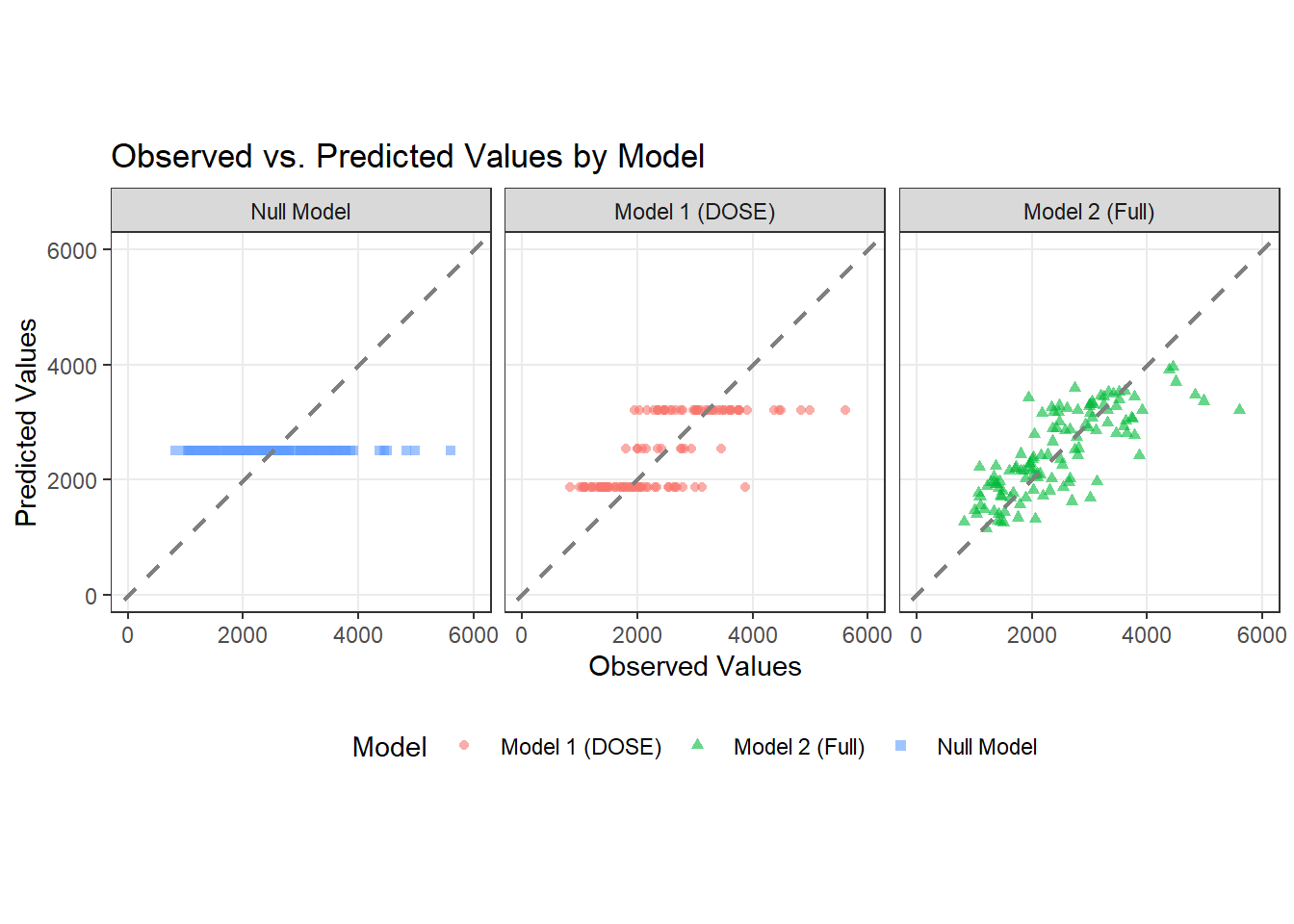
# Plotting observed vs predicted
ggplot(pred_long_format, aes(x = Y, y = prediction, color = model, shape = model)) +
  geom_point(alpha = 0.6, size = 1.5) +
  geom_abline(slope = 1, intercept = 0, color = "gray50", linewidth = 0.8, linetype = "dashed") +
  scale_x_continuous(limits = c(0, 6000)) + # englarged to 6000 because there were values outside the plot
  scale_y_continuous(limits = c(0, 6000)) + # englarged to 6000 because there were values outside the plot
  coord_fixed(ratio = 1) +  # Ensures 45° line appears at true 45°
  labs(
    title = "Observed vs. Predicted Values by Model",
    x = "Observed Values",
    y = "Predicted Values",
    color = "Model",
    shape = "Model"
  ) +
  theme_bw() +
  theme(
    panel.grid.minor = element_blank(),
    legend.position = "bottom"
  ) +
  facet_wrap(~ factor(model,
  levels = c("Null Model", "Model 1 (DOSE)", "Model 2 (Full)")))

#Plotting residuals
data_clean2$residuals_mod2 <- data_clean2$pred_mod2 - data_clean2$Y

ggplot(data_clean2, aes(x = Y, y = residuals_mod2)) + 
  geom_point() +
  geom_abline(slope = 0, intercept = 0, color = "gray50", linewidth = 0.8, linetype = "dashed") +
  ylim(-2000, 2000) + #only 1 value left out to make it more visible
  theme_bw() 

Warning: Removed 1 row containing missing values or values outside the scale range
(`geom_point()`).

set.seed(rngseed) #seed set as rngseed

# Create 100 bootstrap samples from training data
dat_bs <- bootstraps(train_data, times = 100) 

num_obs <- nrow(train_data)
pred_bs <- matrix(NA, nrow = 100, ncol = num_obs)

for (i in 1:100) {
  # Get the i-th bootstrap sample
  dat_sample <- rsample::analysis(dat_bs$splits[[i]])
  
  # Fit the model (Model 2: all predictors) to this sample
  bs_fit <- linear_reg() |> 
    set_engine("lm") |> 
    fit(Y ~ DOSE + AGE + SEX + WT + HT, data = dat_sample)
  
  # Predict for the ORIGINAL training data
  # Use pull(.pred) to get a numeric vector instead of a dataframe
  pred_bs[i, ] <- predict(bs_fit, new_data = dat_sample) |> pull(.pred)
}

preds <- pred_bs |> apply(2, quantile, c(0.055, 0.5, 0.945)) |> t()

# Get the original predictions from the Model 2 fit on training data

aug_train <- augment(new_model2, new_data = train_data)

# Combine with the bootstrap results (the 'preds' matrix from the previous step)
# This assumes 'preds' has columns for 5.5%, 50%, and 94.5% quantiles
plot_data <- aug_train |>
  mutate(
    bs_low = preds[, 1],
    bs_med = preds[, 2],
    bs_high = preds[, 3]
  )

#Plotting the bootstrap results

ggplot(plot_data, aes(x = Y)) +
  # 45-degree reference line (Ideal model)
  geom_abline(intercept = 0, slope = 1, linetype = "dashed", color = "grey50") +
  # Bootstrap intervals (Upper and Lower bounds)
  geom_errorbar(aes(ymin = bs_low, ymax = bs_high), color = "skyblue", alpha = 0.5) +
  # Bootstrap median
  geom_point(aes(y = bs_med), color = "blue", size = 1, alpha = 0.6) +
  # Original point estimate (Original predictions)
  geom_point(aes(y = .pred), color = "black", shape = 1, size = 2) +
  # Formatting
  labs(
    x = "Observed Values",
    y = "Predicted Values (Point & Bootstrap Bounds)",
    title = "Observed vs. Predicted with Bootstrap Uncertainty"
  ) +
  # Ensure x and y axes are on the same scale
  coord_obs_pred() + 
  theme_bw()