Descriptive analysis script by Marco Reina

Code originally written by MR and improve with ChatGPT & Qween

# Load libraries
library(tidyverse)

── Attaching core tidyverse packages ──────────────────────── tidyverse 2.0.0 ──
✔ dplyr     1.1.4     ✔ readr     2.2.0
✔ forcats   1.0.1     ✔ stringr   1.6.0
✔ ggplot2   3.5.2     ✔ tibble    3.2.1
✔ lubridate 1.9.5     ✔ tidyr     1.3.2
✔ purrr     1.2.1     
── Conflicts ────────────────────────────────────────── tidyverse_conflicts() ──
✖ dplyr::filter() masks stats::filter()
✖ dplyr::lag()    masks stats::lag()
ℹ Use the conflicted package (<http://conflicted.r-lib.org/>) to force all conflicts to become errors

library(readr)
library(here)

here() starts at C:/Users/marco/Documents/marcoreina-MADA-project

library(dplyr)
library(stringr)
library(knitr)
library(forcats) 
library(tidytext)

# Read data
isolates1 <- read_csv(here("data/processed-data/", "isolates1.csv"))

Rows: 245772 Columns: 9
── Column specification ────────────────────────────────────────────────────────
Delimiter: ","
chr  (7): Location, Isolation.source, Source.type, BioSample, AMR.genotypes,...
dbl  (1): year
dttm (1): Create.date

ℹ Use `spec()` to retrieve the full column specification for this data.
ℹ Specify the column types or set `show_col_types = FALSE` to quiet this message.

# Get the total number of isolates
totaln_isolates <- nrow(isolates1)

#Split computed serovars
isolates1 <- isolates1 %>%
  mutate(
    antigen_formula = str_extract(Computed.types, "(?<=antigen_formula=).*?(?=,serotype=)"),
    serotype = str_extract(Computed.types, "(?<=serotype=).*$")
  )

# Removing columns that are no longer useful after the original cleaning
isolates1$Computed.types    =   NULL
isolates1$Location  =   NULL
isolates1$country_name  =   NULL

The goal of this analysis is to characterize AMR incidence in Salmonella

As the data comes from an observational surveillance program, only descriptive analysis will be performed. This approach has changed from the original intention described in the manuscript.

#Split AMR genes
amr_long <- isolates1 %>%
  # Keep isolates even if no AMR genes
  mutate(AMR.genotypes = if_else(
    is.na(AMR.genotypes) | AMR.genotypes == "",
    "None=NONE",
    AMR.genotypes
  )) %>%
  # Split genes into rows
  separate_rows(AMR.genotypes, sep = ",")

# Assign antimicrobial class

amr_long <- amr_long %>%
   mutate(
      AMR_class = case_when(
      # === 1. No AMR ===
      str_detect(AMR.genotypes, "None") ~ "No AMR",
      
      # === 2. Beta-lactams ===
      str_detect(AMR.genotypes, "^bla") ~ "Beta_lactam",
      
      # === 3. Tetracyclines ===
      str_detect(AMR.genotypes, "tet") ~ "Tetracycline",
      
      # === 4. Sulfonamides ===
      str_detect(AMR.genotypes, "^sul") ~ "Sulfonamide",
      
      # === 5. Trimethoprim ===
      str_detect(AMR.genotypes, "^dfr") ~ "Trimethoprim",
      
      # === 6. Quinolones: target mutations & protection proteins ===
      str_detect(AMR.genotypes, "gyrA|gyrB|parC_|parE_|^qnr|^oqx|^qepA") ~ "Quinolone",
      
      # === 7. Aminoglycosides: modifying enzymes (broadened) ===
      str_detect(AMR.genotypes, "aad|aph\\(|aac\\(|armA|^rmt|^ant|^aphA|^aacA") ~ "Aminoglycoside",
      
      # === 8. Phenicols (chloramphenicol family) ===
      str_detect(AMR.genotypes, "floR|^cat|^cml|^gar") ~ "Phenicol",  
      
      # === 9. Macrolides: including esterases (estT/estX) ===
      str_detect(AMR.genotypes, "erm|^mef|^mph|^msr|^ere|^est") ~ "Macrolide",  

      # === 10. Lincosamides ===
      str_detect(AMR.genotypes, "^lnu") ~ "Lincosamide",
      
      # === 11. Fosfomycin ===
      str_detect(AMR.genotypes, "^fos") ~ "Fosfomycin",
      
      # === 12. Colistin/Polymyxin: mcr enzymes + pmr regulators ===
      str_detect(AMR.genotypes, "^mcr|^pmrA_|^pmrB_") ~ "Colistin",  
      
      # === 13. Glycopeptides ===
      str_detect(AMR.genotypes, "^van") ~ "Glycopeptide",
      
      # === 14. Rifamycins ===
      str_detect(AMR.genotypes, "^arr") ~ "Rifamycin",
      
      # === 15. Bleomycin resistance ===
      str_detect(AMR.genotypes, "^ble") ~ "Bleomycin",  
      
      # === 16. Streptothricin resistance ===
      str_detect(AMR.genotypes, "^sat") ~ "Streptothricin",  

      # === 17. Streptogramin/Virginiamycin resistance ===
      str_detect(AMR.genotypes, "^vat") ~ "Streptogramin", 
      
      # === 18. Multidrug Efflux Pumps (RND family + tmex/toprJ) ===
      str_detect(AMR.genotypes, "^mds|^acr|^mex|^ade|^cme|^amrB|^tmex|^toprJ") ~ "Efflux Pump",
      
      # === 19. MDR Transcriptional Regulators (upregulate efflux) ===
      str_detect(AMR.genotypes, "^ramR_|^soxR_|^marR|^rob") ~ "MDR Regulator",

      # === 20. Gentamicin ===
      str_detect(AMR.genotypes, "grd") ~ "Gentamicin",
           
      # === 21. Default ===
      TRUE ~ "Other"
    )
  )

# Splitting AMR genes and their status

amr_long <- amr_long %>%
   mutate(
    AMR_gene = str_extract(AMR.genotypes, "^[^=]+"),  # e.g., "aacA56=COMPLETE" → "aacA56"
    AMR_status = str_extract(AMR.genotypes, "(?<==).*") #it keeps the information after "="
   )   

#Removing AMR genotypes after split
amr_long$AMR.genotypes  =   NULL 

#Saving the new data
write_csv(amr_long, here("data/processed-data/", "amr_long.csv"))

AMR summaries

# Gene prevalence overall
gene_prev <- amr_long %>%
  group_by(AMR_gene, AMR_status) %>%
  summarise(n = n(), .groups = "drop") 

write_csv(gene_prev, here("data/processed-data/", "gene_prev.csv"))

gene_prev

# A tibble: 514 × 3
   AMR_gene    AMR_status                n
   <chr>       <chr>                 <int>
 1 None        NONE                   6688
 2 aac(2')-IIa COMPLETE                 86
 3 aac(3)-C322 COMPLETE                  4
 4 aac(3)-I    PARTIAL                   1
 5 aac(3)-II   MISTRANSLATION            1
 6 aac(3)-II   PARTIAL_END_OF_CONTIG     8
 7 aac(3)-IId  COMPLETE                824
 8 aac(3)-IId  MISTRANSLATION            2
 9 aac(3)-IId  PARTIAL                   1
10 aac(3)-IId  PARTIAL_END_OF_CONTIG    12
# ℹ 504 more rows

# Class prevalence overall
class_prev <- amr_long %>%  
  filter(AMR_status == "COMPLETE") %>%  
  group_by(AMR_class) %>%  
  summarise(n = n_distinct(BioSample), .groups = "drop") %>%  
  arrange(desc(n)) %>%  
  mutate(
    Percentage = round(n / totaln_isolates * 100, 1) 
  )

class_prev

# A tibble: 17 × 3
   AMR_class           n Percentage
   <chr>           <int>      <dbl>
 1 Efflux Pump    236114       96.1
 2 Tetracycline    26572       10.8
 3 Aminoglycoside  24171        9.8
 4 Sulfonamide     20618        8.4
 5 Beta_lactam     17522        7.1
 6 Phenicol        10132        4.1
 7 Quinolone        8535        3.5
 8 Trimethoprim     8131        3.3
 9 Fosfomycin       6015        2.4
10 Macrolide        3377        1.4
11 Lincosamide       653        0.3
12 Rifamycin         556        0.2
13 Bleomycin         542        0.2
14 Colistin          485        0.2
15 Gentamicin         53        0  
16 Streptothricin     33        0  
17 Glycopeptide        1        0

# Plotting classes frequencies
ggplot(class_prev, aes(x = fct_reorder(AMR_class, n), y = n)) + 
  geom_col() +  
  coord_flip() +  
  theme_bw()

The vast majority of AMR predicted genes are efflux pumps. I have decided to delete them because it would influence the overall AMR analysis. ¨Several studies show that overexpression of efflux pumps rarely provides clinical resistance but contributes to a low-level resistance.¨ https://doi.org/10.3390/antibiotics9120855 Therefore, while technically AMR, it is so widespread that it should not be considered as a factor for higher risk of developing AMR if already over 90% of isolates show to have it.

# Removing Efflux pumps
amr_long1 <- amr_long[!(amr_long$AMR_class %in% "Efflux Pump"), ]

# Keeping only completed profiles
amr_long1 <- amr_long1[(amr_long1$AMR_status %in% "COMPLETE"), ]

# Class prevalence after removing Efflux pumps and keeping only completed profiles
class_prev1 <- amr_long1 %>%
  group_by(AMR_class) %>%  
  summarise(n = n_distinct(BioSample), .groups = "drop") %>%  
  arrange(desc(n)) %>%  
  mutate(
    Percentage = round(n / totaln_isolates * 100, 1)          
  )

class_prev1

# A tibble: 16 × 3
   AMR_class          n Percentage
   <chr>          <int>      <dbl>
 1 Tetracycline   26572       10.8
 2 Aminoglycoside 24171        9.8
 3 Sulfonamide    20618        8.4
 4 Beta_lactam    17522        7.1
 5 Phenicol       10132        4.1
 6 Quinolone       8535        3.5
 7 Trimethoprim    8131        3.3
 8 Fosfomycin      6015        2.4
 9 Macrolide       3377        1.4
10 Lincosamide      653        0.3
11 Rifamycin        556        0.2
12 Bleomycin        542        0.2
13 Colistin         485        0.2
14 Gentamicin        53        0  
15 Streptothricin    33        0  
16 Glycopeptide       1        0

write_csv(class_prev1, here("data/processed-data/", "class_prev1csv"))

# Plotting classes frequencies after removing Efflux pumps and keeping only completed profiles
ggplot(class_prev1, aes(x = fct_reorder(AMR_class, n), y = n)) + 
  geom_col() +  
  coord_flip() +  
  theme_bw()

#Saving file
ggsave(filename = "amr_graph1.png", path = here("results/figures/"))

Saving 7 x 5 in image

This indicates that most prevalent drug resistant classes are in Salmonella are: Tetracycline, Aminoglycoside, Sulfonamide, Beta-lactam, Phenicol, Quinolone, Trimethoprim, Fosfomycin.

# Create the count of AMR classes
amr_count <- amr_long1 %>%
  filter(AMR_gene != "None") %>%
  distinct(BioSample, AMR_class) %>% 
  count(BioSample, name = "n_classes")

# Join and Mutate to original dataset
isolates1 <- isolates1 %>%
  left_join(amr_count, by = "BioSample") %>%
  mutate(n_classes = tidyr::replace_na(n_classes, 0))

amr_nclasses <- isolates1 %>%
  group_by(n_classes) %>%
  summarise(n = n(), .groups = "drop") 

amr_nclasses

# A tibble: 13 × 2
   n_classes      n
       <int>  <int>
 1         0 207263
 2         1  11317
 3         2   6020
 4         3   4187
 5         4   5876
 6         5   5621
 7         6   1685
 8         7   1094
 9         8   2380
10         9    241
11        10     76
12        11     10
13        12      2

#Creating a variable based on n_classes 
isolates1 <- isolates1 %>%
  mutate(
    MDR_category = case_when(
      n_classes == 0 ~ "0",
      n_classes == 1 ~ "1",
      n_classes == 2 ~ "2",
      n_classes >= 3 ~ "3+",
    ),
    MDR_category = factor(MDR_category, levels = c("0", "1", "2", "3+"), ordered = TRUE)
  )

# Plot AMR by number of classes
  ggplot(isolates1, aes(x = MDR_category)) + 
  geom_bar() +
  theme_bw() +
  facet_wrap(~ Source.type, scales = "free")

ggsave(filename = "amr_graph2.png", path = here("results/figures/"))

Saving 7 x 5 in image

While the scales are different, it is interesting to observe that the trends between environmental and human AMR look very familiar. While the AMR between animal and food resemble also look similar to each other. Proportionally, there are more isolates with MDR observed in animal and food sources. However, we have to take in consideration this is only observational data.

# Creating a wide version for understanding cooccurrance
amr_wide <- amr_long1 %>%
  filter(AMR_gene != "None") %>%
  # Keep only the columns needed for the pivot + identifiers
  select(BioSample, AMR_class, serotype, Source.type) %>%
  # Remove duplicate BioSample + AMR_class combinations while preserving metadata
  distinct(BioSample, .keep_all = TRUE) %>%
  mutate(present = 1) %>%
  pivot_wider(
    id_cols = c(BioSample, serotype, Source.type),
    names_from = AMR_class,
    values_from = present,
    values_fill = 0
  )

amr_order <- c(
  "Tetracycline", "Aminoglycoside", "Sulfonamide", "Beta_lactam", "Phenicol", "Quinolone", "Trimethoprim", "Fosfomycin", "Macrolide", "Lincosamide", "Rifamycin", "Bleomycin", "Colistin", "Gentamicin", "Streptothricin", "Glycopeptide"
)

#AMR matrix full dataset
amr_mat <- amr_wide %>%
  select(-BioSample) %>%   
  select(where(is.numeric)) %>%
  as.matrix()

#Correlation matrix
cor_mat <- cor(amr_mat)
cor_mat

               Aminoglycoside   Fosfomycin    Quinolone Tetracycline
Aminoglycoside     1.00000000 -0.443250155 -0.344475402 -0.321335781
Fosfomycin        -0.44325016  1.000000000 -0.090637634 -0.084549187
Quinolone         -0.34447540 -0.090637634  1.000000000 -0.065708076
Tetracycline      -0.32133578 -0.084549187 -0.065708076  1.000000000
Sulfonamide       -0.16616898 -0.043722029 -0.033978925 -0.031696441
Beta_lactam       -0.36254002 -0.095390758 -0.074133690 -0.069153871
Gentamicin        -0.01750098 -0.004604820 -0.003578672 -0.003338281
Trimethoprim      -0.28446859 -0.074848770 -0.058169320 -0.054261883
Phenicol          -0.10449671 -0.027494953 -0.021367922 -0.019932564
Colistin          -0.03743082 -0.009848717 -0.007654009 -0.007139862
Macrolide         -0.06351658 -0.016712348 -0.012988135 -0.012115676
Bleomycin         -0.01870957 -0.004922823 -0.003825812 -0.003568818
Lincosamide       -0.01322898 -0.003480781 -0.002705117 -0.002523405
                Sulfonamide  Beta_lactam    Gentamicin Trimethoprim
Aminoglycoside -0.166168985 -0.362540021 -0.0175009769 -0.284468592
Fosfomycin     -0.043722029 -0.095390758 -0.0046048198 -0.074848770
Quinolone      -0.033978925 -0.074133690 -0.0035786725 -0.058169320
Tetracycline   -0.031696441 -0.069153871 -0.0033382805 -0.054261883
Sulfonamide     1.000000000 -0.035760812 -0.0017262898 -0.028059875
Beta_lactam    -0.035760812  1.000000000 -0.0037663415 -0.061219775
Gentamicin     -0.001726290 -0.003766341  1.0000000000 -0.002955276
Trimethoprim   -0.028059875 -0.061219775 -0.0029552761  1.000000000
Phenicol       -0.010307517 -0.022488477 -0.0010855913 -0.017645680
Colistin       -0.003692162 -0.008055393 -0.0003888598 -0.006320699
Macrolide      -0.006265252 -0.013669245 -0.0006598586 -0.010725632
Bleomycin      -0.001845505 -0.004026441 -0.0001943693 -0.003159364
Lincosamide    -0.001304902 -0.002846976 -0.0001374327 -0.002233892
                   Phenicol      Colistin     Macrolide     Bleomycin
Aminoglycoside -0.104496714 -0.0374308170 -0.0635165817 -0.0187095742
Fosfomycin     -0.027494953 -0.0098487169 -0.0167123477 -0.0049228233
Quinolone      -0.021367922 -0.0076540090 -0.0129881347 -0.0038258115
Tetracycline   -0.019932564 -0.0071398624 -0.0121156761 -0.0035688183
Sulfonamide    -0.010307517 -0.0036921618 -0.0062652519 -0.0018455054
Beta_lactam    -0.022488477 -0.0080553926 -0.0136692448 -0.0040264407
Gentamicin     -0.001085591 -0.0003888598 -0.0006598586 -0.0001943693
Trimethoprim   -0.017645680 -0.0063206986 -0.0107256320 -0.0031593641
Phenicol        1.000000000 -0.0023218459 -0.0039399544 -0.0011605610
Colistin       -0.002321846  1.0000000000 -0.0014112952 -0.0004157140
Macrolide      -0.003939954 -0.0014112952  1.0000000000 -0.0007054276
Bleomycin      -0.001160561 -0.0004157140 -0.0007054276  1.0000000000
Lincosamide    -0.000820598 -0.0002939389 -0.0004987868 -0.0001469236
                 Lincosamide
Aminoglycoside -0.0132289796
Fosfomycin     -0.0034807809
Quinolone      -0.0027051167
Tetracycline   -0.0025234046
Sulfonamide    -0.0013049016
Beta_lactam    -0.0028469756
Gentamicin     -0.0001374327
Trimethoprim   -0.0022338917
Phenicol       -0.0008205980
Colistin       -0.0002939389
Macrolide      -0.0004987868
Bleomycin      -0.0001469236
Lincosamide     1.0000000000

cor_df <- as.data.frame(as.table(cor_mat)) %>%
  rename(AMR1 = Var1, AMR2 = Var2, corr = Freq) %>%
  mutate(
    AMR1 = factor(AMR1, levels = amr_order),
    AMR2 = factor(AMR2, levels = amr_order)
  ) %>%
    drop_na()


ggplot(cor_df, aes(AMR1, AMR2, fill = corr)) +
  geom_tile() +
  scale_fill_gradient2(low = "blue", mid = "white", high = "red") +
  theme_bw() +
  theme(axis.text.x = element_text(angle = 45, hjust = 1)) +
  labs(title = "AMR Correlation Heatmap")

From this information we can tell the cooccurrance of AMR genes. For the three biggest categories

> Tetracycline has its strongest relationship with Aminoglycosides and Sulfonamides

> Aminoglycosides has its strongest relationship with Tetracycline and Beta_lactams

> Sulfonamides has its strongest relationship with Aminoglycosides, Tetracycline, and Beta_lactams

Quinolone, Fosfomycin, MDR Regulator, and Streptogramin seem to have a negative correlation with most of the other classes.

> In particular, Quinolone and Fosfomycin seem to most negative correlation between each other

After learning about the MDR and the coocurrance af AMR in all isolates, I am interested in two more things: Is cooccurance the same across sources? and what are the serovars leading each one of the main AMR classes?

# ======= AMR matrix per source: HUMAN =========== #
amr_mat_human <- amr_wide %>%
  filter(Source.type == "human") %>%
  select(-BioSample) %>%   
  select(where(is.numeric)) %>%
  as.matrix()

#Correlation matrix
cor_mat_human <- cor(amr_mat_human) 
cor_mat_human

               Aminoglycoside   Fosfomycin    Quinolone Tetracycline
Aminoglycoside    1.000000000 -0.433313897 -0.354644409 -0.307810473
Fosfomycin       -0.433313897  1.000000000 -0.104336916 -0.090558302
Quinolone        -0.354644409 -0.104336916  1.000000000 -0.074117160
Tetracycline     -0.307810473 -0.090558302 -0.074117160  1.000000000
Sulfonamide      -0.118414448 -0.034837708 -0.028512813 -0.024747444
Beta_lactam      -0.357861010 -0.105283245 -0.086168744 -0.074789398
Gentamicin       -0.006969013 -0.002050294 -0.001678057 -0.001456455
Trimethoprim     -0.281562151 -0.082836006 -0.067796871 -0.058843694
Phenicol         -0.104452587 -0.030730107 -0.025150961 -0.021829553
Colistin         -0.039442858 -0.011604148 -0.009497379 -0.008243166
Macrolide        -0.066211096 -0.019479403 -0.015942857 -0.013837462
Bleomycin        -0.018440101 -0.005425105 -0.004440160 -0.003853798
Lincosamide      -0.009855836 -0.002899602 -0.002373170 -0.002059772
                 Sulfonamide  Beta_lactam    Gentamicin Trimethoprim
Aminoglycoside -0.1184144478 -0.357861010 -6.969013e-03 -0.281562151
Fosfomycin     -0.0348377078 -0.105283245 -2.050294e-03 -0.082836006
Quinolone      -0.0285128133 -0.086168744 -1.678057e-03 -0.067796871
Tetracycline   -0.0247474438 -0.074789398 -1.456455e-03 -0.058843694
Sulfonamide     1.0000000000 -0.028771423 -5.602970e-04 -0.022637123
Beta_lactam    -0.0287714227  1.000000000 -1.693277e-03 -0.068411784
Gentamicin     -0.0005602970 -0.001693277  1.000000e+00 -0.001332256
Trimethoprim   -0.0226371229 -0.068411784 -1.332256e-03  1.000000000
Phenicol       -0.0083978121 -0.025379078 -4.942342e-04 -0.019968054
Colistin       -0.0031711394 -0.009583519 -1.866302e-04 -0.007540236
Macrolide      -0.0053232606 -0.016087458 -3.132884e-04 -0.012657482
Bleomycin      -0.0014825531 -0.004480432 -8.725229e-05 -0.003525168
Lincosamide    -0.0007923926 -0.002394694 -4.663447e-05 -0.001884126
                    Phenicol      Colistin     Macrolide     Bleomycin
Aminoglycoside -0.1044525866 -0.0394428584 -0.0662110957 -1.844010e-02
Fosfomycin     -0.0307301073 -0.0116041480 -0.0194794035 -5.425105e-03
Quinolone      -0.0251509605 -0.0094973787 -0.0159428570 -4.440160e-03
Tetracycline   -0.0218295534 -0.0082431658 -0.0138374616 -3.853798e-03
Sulfonamide    -0.0083978121 -0.0031711394 -0.0053232606 -1.482553e-03
Beta_lactam    -0.0253790781 -0.0095835194 -0.0160874577 -4.480432e-03
Gentamicin     -0.0004942342 -0.0001866302 -0.0003132884 -8.725229e-05
Trimethoprim   -0.0199680536 -0.0075402356 -0.0126574817 -3.525168e-03
Phenicol        1.0000000000 -0.0027972407 -0.0046956123 -1.307750e-03
Colistin       -0.0027972407  1.0000000000 -0.0017731334 -4.938260e-04
Macrolide      -0.0046956123 -0.0017731334  1.0000000000 -8.289653e-04
Bleomycin      -0.0013077501 -0.0004938260 -0.0008289653  1.000000e+00
Lincosamide    -0.0006989642 -0.0002639393 -0.0004430640 -1.233954e-04
                 Lincosamide
Aminoglycoside -9.855836e-03
Fosfomycin     -2.899602e-03
Quinolone      -2.373170e-03
Tetracycline   -2.059772e-03
Sulfonamide    -7.923926e-04
Beta_lactam    -2.394694e-03
Gentamicin     -4.663447e-05
Trimethoprim   -1.884126e-03
Phenicol       -6.989642e-04
Colistin       -2.639393e-04
Macrolide      -4.430640e-04
Bleomycin      -1.233954e-04
Lincosamide     1.000000e+00

cor_df_human <- as.data.frame(as.table(cor_mat_human)) %>%
  rename(AMR1 = Var1, AMR2 = Var2, corr = Freq) %>%
  mutate(
    AMR1 = factor(AMR1, levels = amr_order),
    AMR2 = factor(AMR2, levels = amr_order)
  ) %>%
    mutate(corr = replace_na(corr, 0))
    #drop_na()

ggplot(cor_df_human, aes(AMR1, AMR2, fill = corr)) +
  geom_tile() +
  scale_fill_gradient2(low = "blue", mid = "white", high = "red") +
  theme_bw() +
  theme(axis.text.x = element_text(angle = 45, hjust = 1)) +
  labs(title = "AMR Correlation Heatmap: HUMAN")

# ======= AMR matrix per source: ENVIRONMENTAL =========== #
amr_mat_env <- amr_wide %>%
  filter(Source.type == "environmental") %>%
  select(-BioSample) %>%   
  select(where(is.numeric)) %>%
  as.matrix()

#Correlation matrix
cor_mat_env <- cor(amr_mat_env)

Warning in cor(amr_mat_env): the standard deviation is zero

cor_mat_env

               Aminoglycoside  Fosfomycin   Quinolone Tetracycline  Sulfonamide
Aminoglycoside      1.0000000 -0.56863880 -0.36545301  -0.33192712 -0.174315045
Fosfomycin         -0.5686388  1.00000000 -0.09498736  -0.08627341 -0.045307398
Quinolone          -0.3654530 -0.09498736  1.00000000  -0.05544623 -0.029118177
Tetracycline       -0.3319271 -0.08627341 -0.05544623   1.00000000 -0.026446936
Sulfonamide        -0.1743150 -0.04530740 -0.02911818  -0.02644694  1.000000000
Beta_lactam        -0.1228336 -0.03192650 -0.02051854  -0.01863621 -0.009787004
Gentamicin                 NA          NA          NA           NA           NA
Trimethoprim       -0.3466090 -0.09008949 -0.05789875  -0.05258724 -0.027616746
Phenicol           -0.1228336 -0.03192650 -0.02051854  -0.01863621 -0.009787004
Colistin                   NA          NA          NA           NA           NA
Macrolide                  NA          NA          NA           NA           NA
Bleomycin                  NA          NA          NA           NA           NA
Lincosamide                NA          NA          NA           NA           NA
                Beta_lactam Gentamicin Trimethoprim     Phenicol Colistin
Aminoglycoside -0.122833583         NA  -0.34660903 -0.122833583       NA
Fosfomycin     -0.031926504         NA  -0.09008949 -0.031926504       NA
Quinolone      -0.020518539         NA  -0.05789875 -0.020518539       NA
Tetracycline   -0.018636211         NA  -0.05258724 -0.018636211       NA
Sulfonamide    -0.009787004         NA  -0.02761675 -0.009787004       NA
Beta_lactam     1.000000000         NA  -0.01946053 -0.006896552       NA
Gentamicin               NA          1           NA           NA       NA
Trimethoprim   -0.019460534         NA   1.00000000 -0.019460534       NA
Phenicol       -0.006896552         NA  -0.01946053  1.000000000       NA
Colistin                 NA         NA           NA           NA        1
Macrolide                NA         NA           NA           NA       NA
Bleomycin                NA         NA           NA           NA       NA
Lincosamide              NA         NA           NA           NA       NA
               Macrolide Bleomycin Lincosamide
Aminoglycoside        NA        NA          NA
Fosfomycin            NA        NA          NA
Quinolone             NA        NA          NA
Tetracycline          NA        NA          NA
Sulfonamide           NA        NA          NA
Beta_lactam           NA        NA          NA
Gentamicin            NA        NA          NA
Trimethoprim          NA        NA          NA
Phenicol              NA        NA          NA
Colistin              NA        NA          NA
Macrolide              1        NA          NA
Bleomycin             NA         1          NA
Lincosamide           NA        NA           1

cor_df_env <- as.data.frame(as.table(cor_mat_env)) %>%
  rename(AMR1 = Var1, AMR2 = Var2, corr = Freq)   %>%
  mutate(
    AMR1 = factor(AMR1, levels = amr_order),
    AMR2 = factor(AMR2, levels = amr_order)
  ) %>%
    mutate(corr = replace_na(corr, 0))
    #drop_na() %>%
    #filter(!(AMR1 %in% c("Glycopeptide", "Streptothricin")))

ggplot(cor_df_env, aes(AMR1, AMR2, fill = corr)) +
  geom_tile() +
  scale_fill_gradient2(low = "blue", mid = "white", high = "red") +
  theme_bw() +
  theme(axis.text.x = element_text(angle = 45, hjust = 1)) +
  labs(title = "AMR Correlation Heatmap: ENVIRONMENTAL")

# ======= AMR matrix per source: ANIMAL =========== #
amr_mat_animal <- amr_wide %>%
  filter(Source.type == "animal") %>%
  select(-BioSample) %>%   
  select(where(is.numeric)) %>%
  as.matrix()

#Correlation matrix
cor_mat_animal <- cor(amr_mat_animal)

Warning in cor(amr_mat_animal): the standard deviation is zero

cor_mat_animal

               Aminoglycoside   Fosfomycin    Quinolone Tetracycline
Aminoglycoside     1.00000000 -0.479944937 -0.278578778 -0.475569949
Fosfomycin        -0.47994494  1.000000000 -0.045394617 -0.077494474
Quinolone         -0.27857878 -0.045394617  1.000000000 -0.044980818
Tetracycline      -0.47556995 -0.077494474 -0.044980818  1.000000000
Sulfonamide       -0.24750576 -0.040331246 -0.023409830 -0.039963603
Beta_lactam       -0.31909289 -0.051996422 -0.030180753 -0.051522443
Gentamicin        -0.03465124 -0.005646445 -0.003277417 -0.005594974
Trimethoprim      -0.28083975 -0.045763044 -0.026562658 -0.045345887
Phenicol          -0.07754578 -0.012636142 -0.007334510 -0.012520955
Colistin                   NA           NA           NA           NA
Macrolide         -0.03465124 -0.005646445 -0.003277417 -0.005594974
Bleomycin         -0.03465124 -0.005646445 -0.003277417 -0.005594974
Lincosamide       -0.04901424 -0.007986907 -0.004635913 -0.007914102
                Sulfonamide  Beta_lactam    Gentamicin Trimethoprim
Aminoglycoside -0.247505761 -0.319092889 -0.0346512390 -0.280839751
Fosfomycin     -0.040331246 -0.051996422 -0.0056464449 -0.045763044
Quinolone      -0.023409830 -0.030180753 -0.0032774171 -0.026562658
Tetracycline   -0.039963603 -0.051522443 -0.0055949742 -0.045345887
Sulfonamide     1.000000000 -0.026814355 -0.0029118500 -0.023599826
Beta_lactam    -0.026814355  1.000000000 -0.0037540565 -0.030425703
Gentamicin     -0.002911850 -0.003754057  1.0000000000 -0.003304017
Trimethoprim   -0.023599826 -0.030425703 -0.0033040169  1.000000000
Phenicol       -0.006516410 -0.008401178 -0.0009123087 -0.007394037
Colistin                 NA           NA            NA           NA
Macrolide      -0.002911850 -0.003754057 -0.0004076641 -0.003304017
Bleomycin      -0.002911850 -0.003754057 -0.0004076641 -0.003304017
Lincosamide    -0.004118817 -0.005310120 -0.0005766416 -0.004673538
                    Phenicol Colistin     Macrolide     Bleomycin   Lincosamide
Aminoglycoside -0.0775457770       NA -0.0346512390 -0.0346512390 -0.0490142439
Fosfomycin     -0.0126361415       NA -0.0056464449 -0.0056464449 -0.0079869072
Quinolone      -0.0073345099       NA -0.0032774171 -0.0032774171 -0.0046359127
Tetracycline   -0.0125209555       NA -0.0055949742 -0.0055949742 -0.0079141017
Sulfonamide    -0.0065164097       NA -0.0029118500 -0.0029118500 -0.0041188174
Beta_lactam    -0.0084011781       NA -0.0037540565 -0.0037540565 -0.0053101202
Gentamicin     -0.0009123087       NA -0.0004076641 -0.0004076641 -0.0005766416
Trimethoprim   -0.0073940375       NA -0.0033040169 -0.0033040169 -0.0046735382
Phenicol        1.0000000000       NA -0.0009123087 -0.0009123087 -0.0012904625
Colistin                  NA        1            NA            NA            NA
Macrolide      -0.0009123087       NA  1.0000000000 -0.0004076641 -0.0005766416
Bleomycin      -0.0009123087       NA -0.0004076641  1.0000000000 -0.0005766416
Lincosamide    -0.0012904625       NA -0.0005766416 -0.0005766416  1.0000000000

cor_df_animal <- as.data.frame(as.table(cor_mat_animal)) %>%
  rename(AMR1 = Var1, AMR2 = Var2, corr = Freq) %>%
  mutate(
    AMR1 = factor(AMR1, levels = amr_order),
    AMR2 = factor(AMR2, levels = amr_order)
  ) %>%
    mutate(corr = replace_na(corr, 0))
    #drop_na() %>%
    #filter(!(AMR1 %in% c("Glycopeptide", "Streptothricin")))

ggplot(cor_df_animal, aes(AMR1, AMR2, fill = corr)) +
  geom_tile() +
  scale_fill_gradient2(low = "blue", mid = "white", high = "red") +
  theme_bw() +
  theme(axis.text.x = element_text(angle = 45, hjust = 1)) +
  labs(title = "AMR Correlation Heatmap: ANIMAL")

# ======= AMR matrix per source: FOOD =========== #
amr_mat_food <- amr_wide %>%
  filter(Source.type == "food") %>%
  select(-BioSample) %>%   
  select(where(is.numeric)) %>%
  as.matrix()

#Correlation matrix
cor_mat_food <- cor(amr_mat_food, use = "pairwise.complete.obs")

Warning in cor(amr_mat_food, use = "pairwise.complete.obs"): the standard
deviation is zero

cor_mat_food

               Aminoglycoside   Fosfomycin    Quinolone Tetracycline
Aminoglycoside     1.00000000 -0.458769746 -0.163130712 -0.339449797
Fosfomycin        -0.45876975  1.000000000 -0.024410209 -0.050793871
Quinolone         -0.16313071 -0.024410209  1.000000000 -0.018061436
Tetracycline      -0.33944980 -0.050793871 -0.018061436  1.000000000
Sulfonamide       -0.42255463 -0.063229336 -0.022483276 -0.046784221
Beta_lactam       -0.42174099 -0.063107587 -0.022439984 -0.046694137
Gentamicin        -0.05541498 -0.008292070 -0.002948519 -0.006135412
Trimethoprim      -0.26753991 -0.040033571 -0.014235256 -0.029621368
Phenicol          -0.09607785 -0.014376694 -0.005112108 -0.010637506
Colistin                   NA           NA           NA           NA
Macrolide         -0.02477241 -0.003706842 -0.001318090 -0.002742741
Bleomycin                  NA           NA           NA           NA
Lincosamide                NA           NA           NA           NA
                Sulfonamide  Beta_lactam    Gentamicin Trimethoprim
Aminoglycoside -0.422554627 -0.421740991 -0.0554149849 -0.267539905
Fosfomycin     -0.063229336 -0.063107587 -0.0082920704 -0.040033571
Quinolone      -0.022483276 -0.022439984 -0.0029485191 -0.014235256
Tetracycline   -0.046784221 -0.046694137 -0.0061354124 -0.029621368
Sulfonamide     1.000000000 -0.058125896 -0.0076374973 -0.036873335
Beta_lactam    -0.058125896  1.000000000 -0.0076227912 -0.036802335
Gentamicin     -0.007637497 -0.007622791  1.0000000000 -0.004835671
Trimethoprim   -0.036873335 -0.036802335 -0.0048356714  1.000000000
Phenicol       -0.013241803 -0.013216306 -0.0017365668 -0.008384030
Colistin                 NA           NA            NA           NA
Macrolide      -0.003414225 -0.003407651 -0.0004477509 -0.002161712
Bleomycin                NA           NA            NA           NA
Lincosamide              NA           NA            NA           NA
                    Phenicol Colistin     Macrolide Bleomycin Lincosamide
Aminoglycoside -0.0960778495       NA -0.0247724118        NA          NA
Fosfomycin     -0.0143766941       NA -0.0037068418        NA          NA
Quinolone      -0.0051121077       NA -0.0013180898        NA          NA
Tetracycline   -0.0106375060       NA -0.0027427412        NA          NA
Sulfonamide    -0.0132418030       NA -0.0034142250        NA          NA
Beta_lactam    -0.0132163057       NA -0.0034076509        NA          NA
Gentamicin     -0.0017365668       NA -0.0004477509        NA          NA
Trimethoprim   -0.0083840302       NA -0.0021617121        NA          NA
Phenicol        1.0000000000       NA -0.0007763053        NA          NA
Colistin                  NA       NA            NA        NA          NA
Macrolide      -0.0007763053       NA  1.0000000000        NA          NA
Bleomycin                 NA       NA            NA        NA          NA
Lincosamide               NA       NA            NA        NA          NA

cor_df_food <- as.data.frame(as.table(cor_mat_food)) %>%
  rename(AMR1 = Var1, AMR2 = Var2, corr = Freq) %>%
  mutate(
    AMR1 = factor(AMR1, levels = amr_order),
    AMR2 = factor(AMR2, levels = amr_order)
  ) %>%
    mutate(corr = replace_na(corr, 0))
    #drop_na()

ggplot(cor_df_food, aes(AMR1, AMR2, fill = corr)) +
  geom_tile() +
  scale_fill_gradient2(low = "blue", mid = "white", high = "red") +
  theme_bw() +
  theme(axis.text.x = element_text(angle = 45, hjust = 1)) +
  labs(title = "AMR Correlation Heatmap: FOOD")

From this information we can observe that trends are different among sources. Animal and environmental matrixes resemble closely the correlations observed in human isolates. Also, only human isolates presented Glycopeptide and Streptothricin as predicted AMR classes.

Additional observations:

> The pairs: Gentamicin-Colistin and Rifamycin-Colistin are both infrequent but they seem to cooccur in animal and environmental samples.

> Tetracycline, Aminoglycoside, Sulfonamide, Beta_lactams, and Phenicol are high frequency and cooccurance with each other in human, animal, and environmental samples

> Food isolates have the lowest correlation values among AMR classes

> Fosfomycin has a negative correlation to the majority of AMR classes across all sources

#Plotting top serovars
amr_long1 %>% 
  group_by(serotype) %>%
  summarise(n = n_distinct(BioSample), .groups = "drop") %>%  
  arrange(desc(n)) %>% 
  slice_max(n, n = 5, with_ties = FALSE) %>% 
  ungroup() %>%
  ggplot(aes(x = fct_reorder(serotype, n, .desc = FALSE, .fun = max), 
             y = n, fill = serotype)) + 
  geom_col() +  
  coord_flip() +  
  theme_bw() +
  theme(legend.position = "none")

#Plotting top serovars by each source
amr_long1 %>% 
  group_by(Source.type, serotype) %>%
  summarise(n = n_distinct(BioSample), .groups = "drop") %>%
  group_by(Source.type) %>%
  slice_max(n, n = 5, with_ties = FALSE) %>% 
  ungroup() %>%
  ggplot(aes(x = reorder_within(serotype, n, Source.type), y = n, fill = serotype)) + 
  geom_col() +  
  coord_flip() +  
  theme_bw() +
  facet_wrap(~ Source.type, scales = "free") +
  scale_x_reordered() +
  theme(legend.position = "none")

amr_long1 %>%
  filter(serotype == "I 4,[5],12:i:-") %>%
  group_by(Source.type, AMR_class) %>%
  summarise(n = n_distinct(BioSample), .groups = "drop") %>%
  ggplot(aes(x = fct_reorder(AMR_class, n), y = n)) +
  geom_col() +
  coord_flip() +
  theme_bw() +
  facet_wrap(~ Source.type, scales = "free_x", nrow = 1) +
  labs(title = "I 4,[5],12:i:-")

amr_long1 %>%
  filter(serotype == "Newport") %>%
  group_by(Source.type, AMR_class) %>%
  summarise(n = n_distinct(BioSample), .groups = "drop") %>%
  ggplot(aes(x = fct_reorder(AMR_class, n), y = n)) +
  geom_col() +
  coord_flip() +
  theme_bw() +
  facet_wrap(~ Source.type, scales = "free_x", nrow = 1) +
  labs(title = "Newport")

amr_long1 %>%
  filter(serotype == "Typhimurium") %>%
  group_by(Source.type, AMR_class) %>%
  summarise(n = n_distinct(BioSample), .groups = "drop") %>%
  ggplot(aes(x = fct_reorder(AMR_class, n), y = n)) +
  geom_col() +
  coord_flip() +
  theme_bw() +
  facet_wrap(~ Source.type, scales = "free_x", nrow = 1) +
  labs(title = "Typhimurium")

amr_long1 %>%
  filter(serotype == "Infantis") %>%
  group_by(Source.type, AMR_class) %>%
  summarise(n = n_distinct(BioSample), .groups = "drop") %>%
  ggplot(aes(x = fct_reorder(AMR_class, n), y = n)) +
  geom_col() +
  coord_flip() +
  theme_bw() +
  facet_wrap(~ Source.type, scales = "free_x", nrow = 1) +
  labs(title = "Infantis")

amr_long1 %>%
  filter(serotype == "Dublin") %>%
  group_by(Source.type, AMR_class) %>%
  summarise(n = n_distinct(BioSample), .groups = "drop") %>%
  ggplot(aes(x = fct_reorder(AMR_class, n), y = n)) +
  geom_col() +
  coord_flip() +
  theme_bw() +
  facet_wrap(~ Source.type, scales = "free_x", nrow = 1) +
  labs(title = "Dublin")

amr_long1 %>% 
  filter(AMR_class == "Tetracycline") %>%
  group_by(Source.type, serotype) %>%
  summarise(n = n_distinct(BioSample), .groups = "drop") %>%
  group_by(Source.type) %>%
  slice_max(n, n = 5, with_ties = FALSE) %>% 
  ungroup() %>%
  ggplot(aes(x = reorder_within(serotype, n, Source.type), y = n, fill = serotype)) + 
  geom_col() +  
  coord_flip() +  
  theme_bw() +
  facet_wrap(~ Source.type, scales = "free") +
  scale_x_reordered() +
  theme(legend.position = "none") +
  labs(title = "Tetracycline")

#Now serovar trends will be graph per each one of the AMR classes, while not all of them will be included in the manuscruipt. Maybe as supplemental material.

amr_long1 %>% 
  filter(AMR_class == "Tetracycline") %>%
  group_by(Source.type, serotype) %>%
  summarise(n = n_distinct(BioSample), .groups = "drop") %>%
  group_by(Source.type) %>%
  slice_max(n, n = 5, with_ties = FALSE) %>% 
  ungroup() %>%
  ggplot(aes(x = reorder_within(serotype, n, Source.type), y = n, fill = serotype)) + 
  geom_col() +  
  coord_flip() +  
  theme_bw() +
  facet_wrap(~ Source.type, scales = "free") +
  scale_x_reordered() +
  theme(legend.position = "none") +
  labs(title = "Tetracycline")

amr_long1 %>% 
  filter(AMR_class == "Aminoglycoside") %>%
  group_by(Source.type, serotype) %>%
  summarise(n = n_distinct(BioSample), .groups = "drop") %>%
  group_by(Source.type) %>%
  slice_max(n, n = 5, with_ties = FALSE) %>% 
  ungroup() %>%
  ggplot(aes(x = reorder_within(serotype, n, Source.type), y = n, fill = serotype)) + 
  geom_col() +  
  coord_flip() +  
  theme_bw() +
  facet_wrap(~ Source.type, scales = "free") +
  scale_x_reordered() +
  theme(legend.position = "none") +
  labs(title = "Aminoglycoside")

amr_long1 %>% 
  filter(AMR_class == "Sulfonamide") %>%
  group_by(Source.type, serotype) %>%
  summarise(n = n_distinct(BioSample), .groups = "drop") %>%
  group_by(Source.type) %>%
  slice_max(n, n = 5, with_ties = FALSE) %>% 
  ungroup() %>%
  ggplot(aes(x = reorder_within(serotype, n, Source.type), y = n, fill = serotype)) + 
  geom_col() +  
  coord_flip() +  
  theme_bw() +
  facet_wrap(~ Source.type, scales = "free") +
  scale_x_reordered() +
  theme(legend.position = "none") +
  labs(title = "Sulfonamide")

amr_long1 %>% 
  filter(AMR_class == "Beta_lactam") %>%
  group_by(Source.type, serotype) %>%
  summarise(n = n_distinct(BioSample), .groups = "drop") %>%
  group_by(Source.type) %>%
  slice_max(n, n = 5, with_ties = FALSE) %>% 
  ungroup() %>%
  ggplot(aes(x = reorder_within(serotype, n, Source.type), y = n, fill = serotype)) + 
  geom_col() +  
  coord_flip() +  
  theme_bw() +
  facet_wrap(~ Source.type, scales = "free") +
  scale_x_reordered() +
  theme(legend.position = "none") +
  labs(title = "Beta_lactam")

amr_long1 %>% 
  filter(AMR_class == "Phenicol") %>%
  group_by(Source.type, serotype) %>%
  summarise(n = n_distinct(BioSample), .groups = "drop") %>%
  group_by(Source.type) %>%
  slice_max(n, n = 5, with_ties = FALSE) %>% 
  ungroup() %>%
  ggplot(aes(x = reorder_within(serotype, n, Source.type), y = n, fill = serotype)) + 
  geom_col() +  
  coord_flip() +  
  theme_bw() +
  facet_wrap(~ Source.type, scales = "free") +
  scale_x_reordered() +
  theme(legend.position = "none") +
  labs(title = "Phenicol")

amr_long1 %>% 
  filter(AMR_class == "Quinolone") %>%
  group_by(Source.type, serotype) %>%
  summarise(n = n_distinct(BioSample), .groups = "drop") %>%
  group_by(Source.type) %>%
  slice_max(n, n = 5, with_ties = FALSE) %>% 
  ungroup() %>%
  ggplot(aes(x = reorder_within(serotype, n, Source.type), y = n, fill = serotype)) + 
  geom_col() +  
  coord_flip() +  
  theme_bw() +
  facet_wrap(~ Source.type, scales = "free") +
  scale_x_reordered() +
  theme(legend.position = "none") +
  labs(title = "Quinolone")

amr_long1 %>% 
  filter(AMR_class == "Trimethoprim") %>%
  group_by(Source.type, serotype) %>%
  summarise(n = n_distinct(BioSample), .groups = "drop") %>%
  group_by(Source.type) %>%
  slice_max(n, n = 5, with_ties = FALSE) %>% 
  ungroup() %>%
  ggplot(aes(x = reorder_within(serotype, n, Source.type), y = n, fill = serotype)) + 
  geom_col() +  
  coord_flip() +  
  theme_bw() +
  facet_wrap(~ Source.type, scales = "free") +
  scale_x_reordered() +
  theme(legend.position = "none") +
  labs(title = "Trimethoprim")

amr_long1 %>% 
  filter(AMR_class == "Fosfomycin") %>%
  group_by(Source.type, serotype) %>%
  summarise(n = n_distinct(BioSample), .groups = "drop") %>%
  group_by(Source.type) %>%
  slice_max(n, n = 5, with_ties = FALSE) %>% 
  ungroup() %>%
  ggplot(aes(x = reorder_within(serotype, n, Source.type), y = n, fill = serotype)) + 
  geom_col() +  
  coord_flip() +  
  theme_bw() +
  facet_wrap(~ Source.type, scales = "free") +
  scale_x_reordered() +
  theme(legend.position = "none") +
  labs(title = "Fosfomycin")

amr_long1 %>% 
  filter(AMR_class == "Macrolide") %>%
  group_by(Source.type, serotype) %>%
  summarise(n = n_distinct(BioSample), .groups = "drop") %>%
  group_by(Source.type) %>%
  slice_max(n, n = 5, with_ties = FALSE) %>% 
  ungroup() %>%
  ggplot(aes(x = reorder_within(serotype, n, Source.type), y = n, fill = serotype)) + 
  geom_col() +  
  coord_flip() +  
  theme_bw() +
  facet_wrap(~ Source.type, scales = "free") +
  scale_x_reordered() +
  theme(legend.position = "none") +
  labs(title = "Macrolide")

amr_long1 %>% 
  filter(AMR_class == "Lincosamide") %>%
  group_by(Source.type, serotype) %>%
  summarise(n = n_distinct(BioSample), .groups = "drop") %>%
  group_by(Source.type) %>%
  slice_max(n, n = 5, with_ties = FALSE) %>% 
  ungroup() %>%
  ggplot(aes(x = reorder_within(serotype, n, Source.type), y = n, fill = serotype)) + 
  geom_col() +  
  coord_flip() +  
  theme_bw() +
  facet_wrap(~ Source.type, scales = "free") +
  scale_x_reordered() +
  theme(legend.position = "none") +
  labs(title = "Lincosamide")

amr_long1 %>% 
  filter(AMR_class == "Rifamycin") %>%
  group_by(Source.type, serotype) %>%
  summarise(n = n_distinct(BioSample), .groups = "drop") %>%
  group_by(Source.type) %>%
  slice_max(n, n = 5, with_ties = FALSE) %>% 
  ungroup() %>%
  ggplot(aes(x = reorder_within(serotype, n, Source.type), y = n, fill = serotype)) + 
  geom_col() +  
  coord_flip() +  
  theme_bw() +
  facet_wrap(~ Source.type, scales = "free") +
  scale_x_reordered() +
  theme(legend.position = "none") +
  labs(title = "Rifamycin")

amr_long1 %>% 
  filter(AMR_class == "Bleomycin") %>%
  group_by(Source.type, serotype) %>%
  summarise(n = n_distinct(BioSample), .groups = "drop") %>%
  group_by(Source.type) %>%
  slice_max(n, n = 5, with_ties = FALSE) %>% 
  ungroup() %>%
  ggplot(aes(x = reorder_within(serotype, n, Source.type), y = n, fill = serotype)) + 
  geom_col() +  
  coord_flip() +  
  theme_bw() +
  facet_wrap(~ Source.type, scales = "free") +
  scale_x_reordered() +
  theme(legend.position = "none") +
  labs(title = "Bleomycin")

amr_long1 %>% 
  filter(AMR_class == "Colistin") %>%
  group_by(Source.type, serotype) %>%
  summarise(n = n_distinct(BioSample), .groups = "drop") %>%
  group_by(Source.type) %>%
  slice_max(n, n = 5, with_ties = FALSE) %>% 
  ungroup() %>%
  ggplot(aes(x = reorder_within(serotype, n, Source.type), y = n, fill = serotype)) + 
  geom_col() +  
  coord_flip() +  
  theme_bw() +
  facet_wrap(~ Source.type, scales = "free") +
  scale_x_reordered() +
  theme(legend.position = "none") +
  labs(title = "Colistin")

amr_long1 %>% 
  filter(AMR_class == "Gentamicin") %>%
  group_by(Source.type, serotype) %>%
  summarise(n = n_distinct(BioSample), .groups = "drop") %>%
  group_by(Source.type) %>%
  slice_max(n, n = 5, with_ties = FALSE) %>% 
  ungroup() %>%
  ggplot(aes(x = reorder_within(serotype, n, Source.type), y = n, fill = serotype)) + 
  geom_col() +  
  coord_flip() +  
  theme_bw() +
  facet_wrap(~ Source.type, scales = "free") +
  scale_x_reordered() +
  theme(legend.position = "none") +
  labs(title = "Gentamicin")

amr_long1 %>% 
  filter(AMR_class == "Streptothricin") %>%
  group_by(Source.type, serotype) %>%
  summarise(n = n_distinct(BioSample), .groups = "drop") %>%
  group_by(Source.type) %>%
  slice_max(n, n = 5, with_ties = FALSE) %>% 
  ungroup() %>%
  ggplot(aes(x = reorder_within(serotype, n, Source.type), y = n, fill = serotype)) + 
  geom_col() +  
  coord_flip() +  
  theme_bw() +
  facet_wrap(~ Source.type, scales = "free") +
  scale_x_reordered() +
  theme(legend.position = "none") +
  labs(title = "Streptothricin")

Publication ready Figures and tables

library(gt)

# Publication-ready Table for Class Prevalence
class_prev1 %>%
  gt() %>%
  tab_header(
    title = "Prevalence of Clinically Relevant AMR Classes",
    subtitle = "Excluding Efflux Pumps; (n = 245,772 isolates)"
  ) %>%
  cols_label(
    AMR_class = "Antimicrobial Class",
    n = "Isolate Count",
    Percentage = "Prevalence (%)"
  ) %>%
  fmt_number(columns = n, decimals = 0, use_seps = TRUE) %>%
  data_color(
    columns = Percentage,
    palette = "YlOrRd",
    domain = c(0, 12)
  ) %>%
  opt_stylize(style = 1, color = "gray") %>%
  gtsave(here("results/tables/amr_class_prevalence.html"))

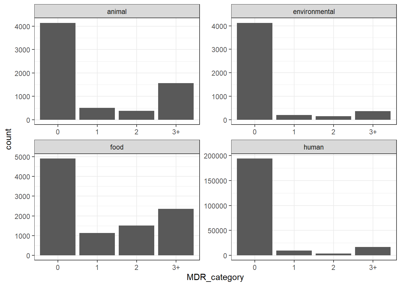
# Publication-ready MDR Plot
ggplot(isolates1, aes(x = MDR_category, fill = MDR_category)) +
  geom_bar(show.legend = FALSE) +
  facet_wrap(~ Source.type, scales = "free_y") +
  scale_fill_brewer(palette = "Blues") +
  labs(
    title = "Distribution of Multidrug Resistance (MDR) by Source",
    subtitle = "Categories: 0, 1, 2, or 3+ resistance classes",
    x = "Number of Resistance Classes",
    y = "Isolate Count"
  ) +
  theme_bw() +
  theme(strip.background = element_rect(fill = "white"),
        strip.text = element_text(face = "bold")) -> amr_graph2_pub

ggsave(here("results/figures/amr_mdr_distribution.png"), plot = amr_graph2_pub, dpi = 300, width = 8, height = 6)

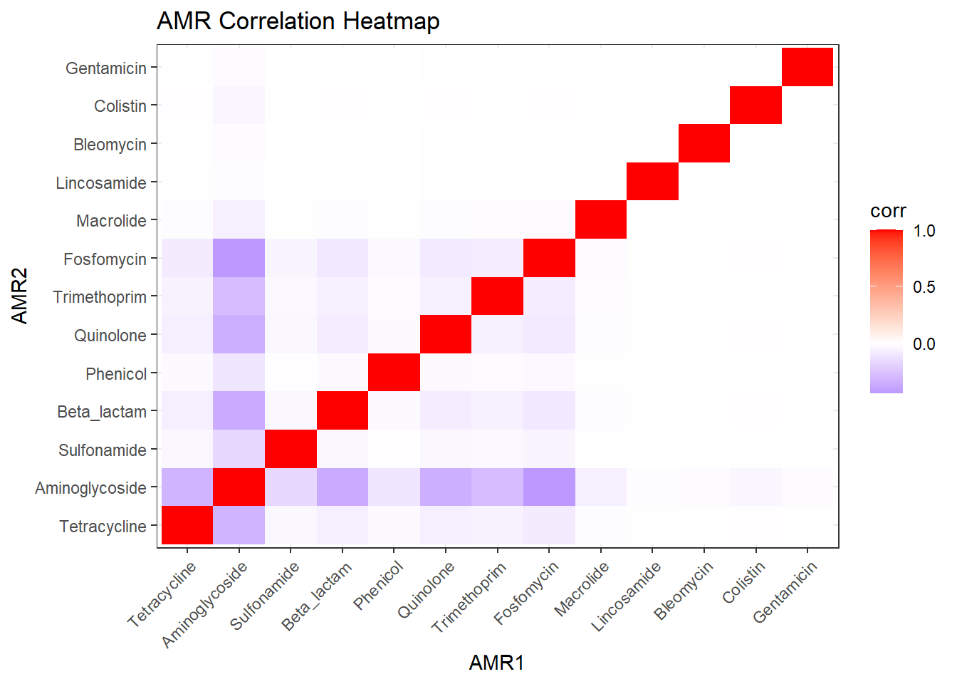
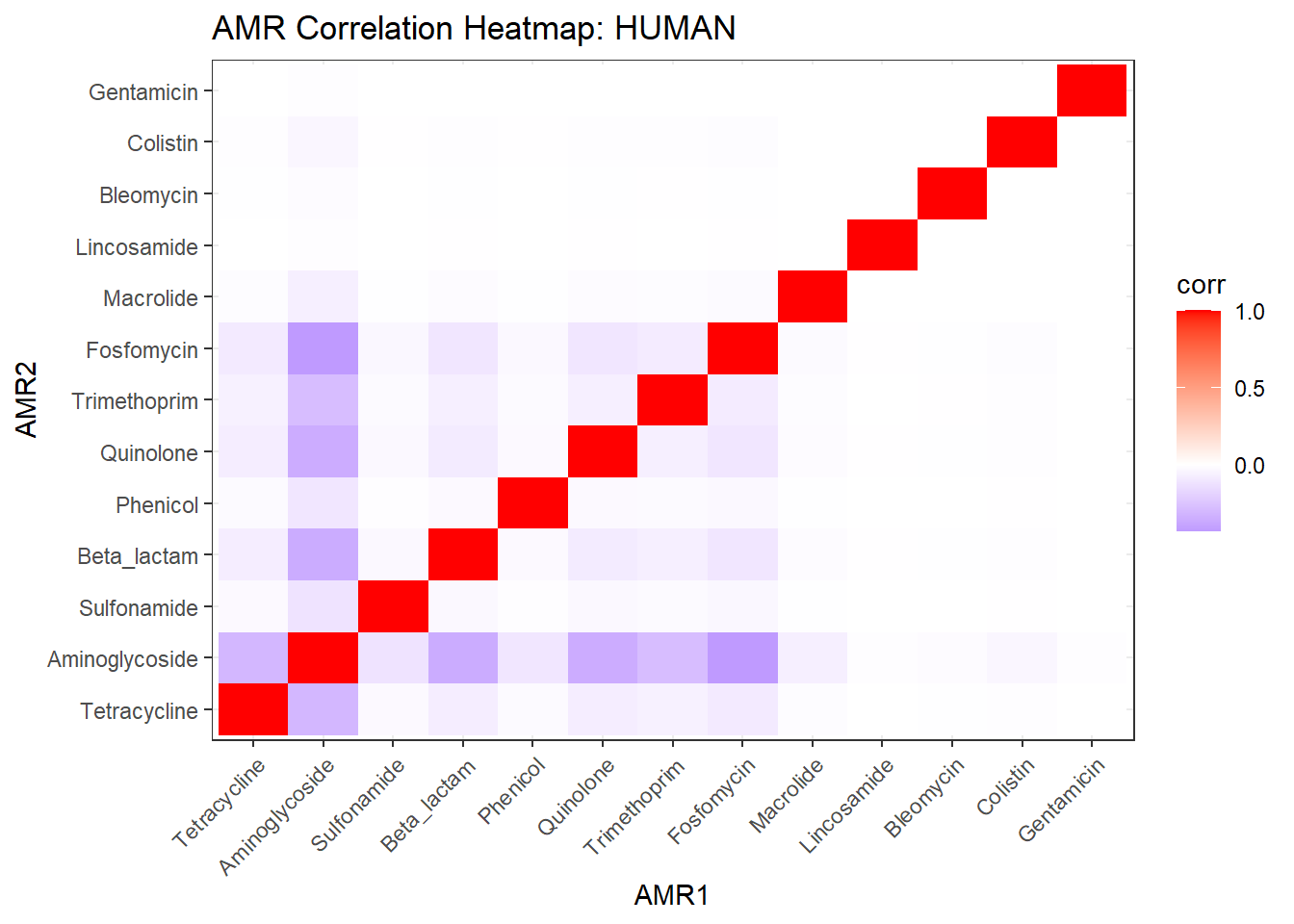
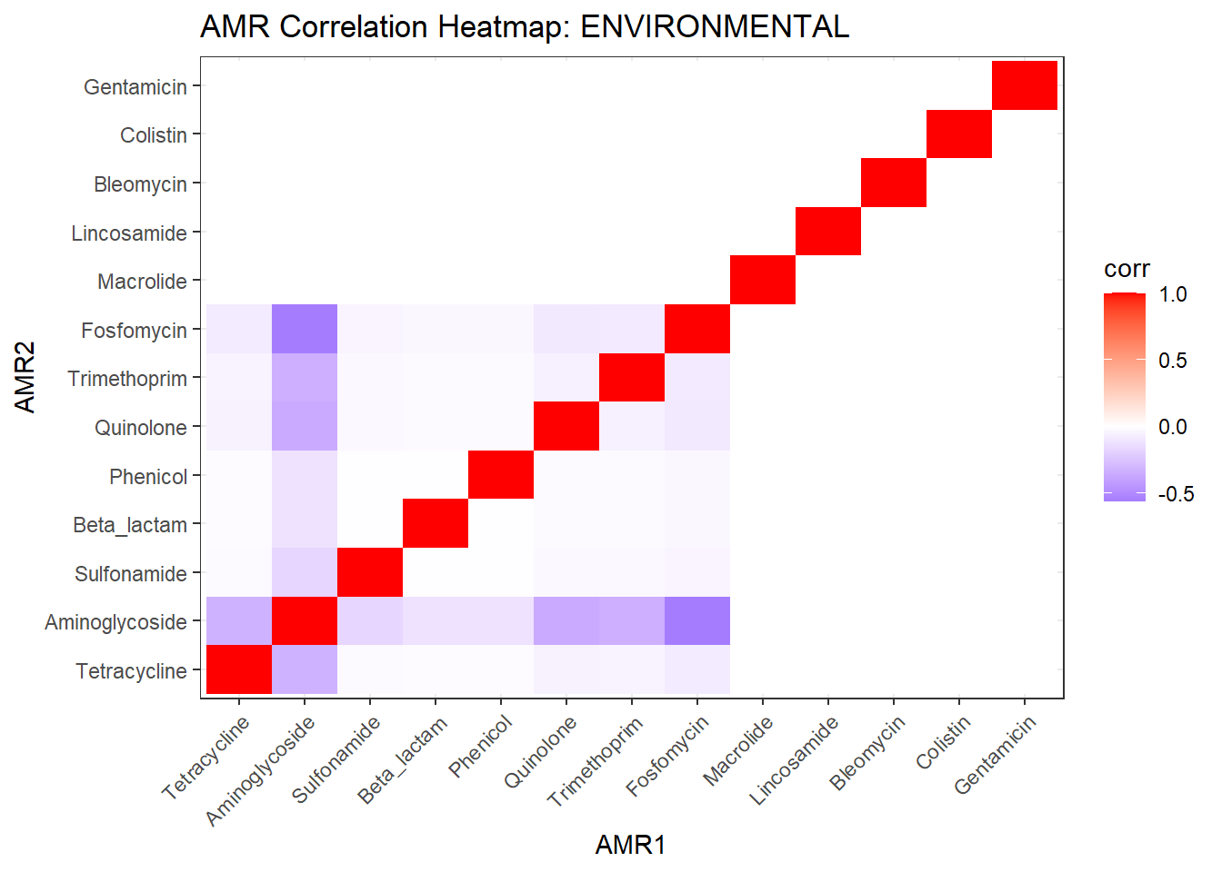
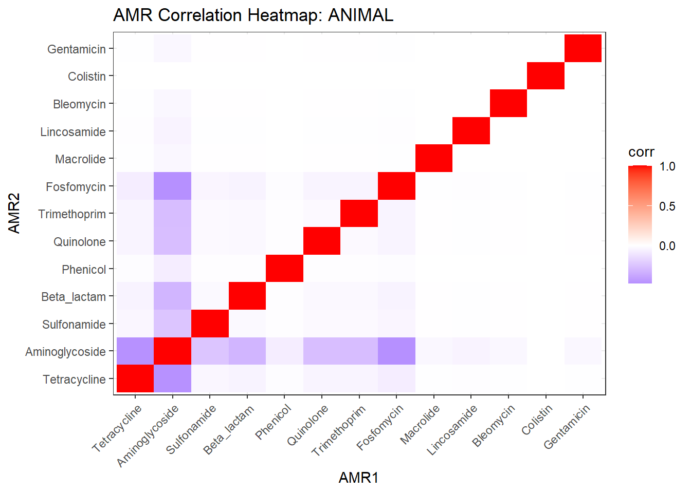
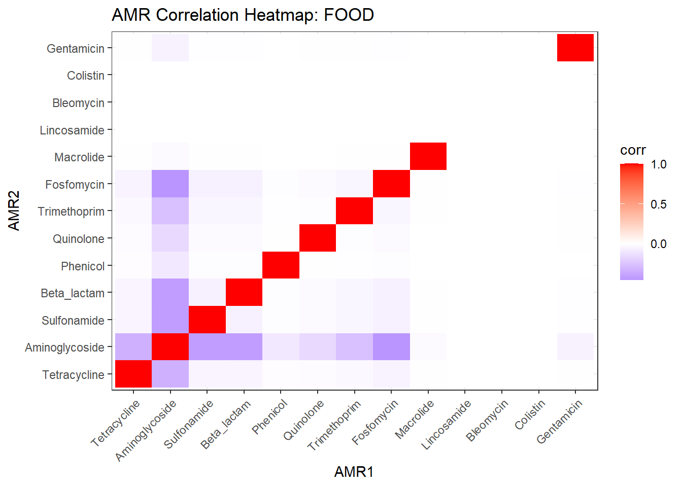
# Publication-ready Heatmap
ggplot(cor_df, aes(AMR1, AMR2, fill = corr)) +
  geom_tile(color = "white") +
  scale_fill_gradient2(low = "#2166ac", mid = "#f7f7f7", high = "#b2182b", 
                       midpoint = 0, limit = c(-1, 1), name = "Pearson\nCorr") +
  theme_minimal() +
  theme(axis.text.x = element_text(angle = 45, vjust = 1, hjust = 1),
        panel.grid.major = element_blank()) +
  labs(title = "Co-occurrence of Antimicrobial Resistance Classes",
       x = NULL, y = NULL) -> amr_heatmap_pub

ggsave(here("results/figures/amr_correlation_heatmap.png"), plot = amr_heatmap_pub, dpi = 300, width = 9, height = 7)