MODEL FITTING

Using second dataset: “Genomes”

library(tidyverse)   

── Attaching core tidyverse packages ──────────────────────── tidyverse 2.0.0 ──
✔ dplyr     1.1.4     ✔ readr     2.2.0
✔ forcats   1.0.1     ✔ stringr   1.6.0
✔ ggplot2   3.5.2     ✔ tibble    3.2.1
✔ lubridate 1.9.5     ✔ tidyr     1.3.2
✔ purrr     1.2.1     
── Conflicts ────────────────────────────────────────── tidyverse_conflicts() ──
✖ dplyr::filter() masks stats::filter()
✖ dplyr::lag()    masks stats::lag()
ℹ Use the conflicted package (<http://conflicted.r-lib.org/>) to force all conflicts to become errors

library(tidymodels) 

── Attaching packages ────────────────────────────────────── tidymodels 1.4.1 ──
✔ broom        1.0.12     ✔ rsample      1.3.2 
✔ dials        1.4.2      ✔ tailor       0.1.0 
✔ infer        1.1.0      ✔ tune         2.0.1 
✔ modeldata    1.5.1      ✔ workflows    1.3.0 
✔ parsnip      1.4.1      ✔ workflowsets 1.1.1 
✔ recipes      1.3.1      ✔ yardstick    1.3.2 
── Conflicts ───────────────────────────────────────── tidymodels_conflicts() ──
✖ scales::discard() masks purrr::discard()
✖ dplyr::filter()   masks stats::filter()
✖ recipes::fixed()  masks stringr::fixed()
✖ dplyr::lag()      masks stats::lag()
✖ yardstick::spec() masks readr::spec()
✖ recipes::step()   masks stats::step()

library(here)        

here() starts at C:/Users/marco/Documents/marcoreina-MADA-project

#Load files created data has been previously cleaned
genomes1 <- read.csv(here("data/processed-data/", "genomes1.csv")) %>% 
  mutate(Annotation.Release.Date = as.Date(Annotation.Release.Date)) %>% 
  group_by(BioSample) %>% 
  filter(Annotation.Release.Date== max(Annotation.Release.Date, na.rm = TRUE)) %>% 
  ungroup()

write_csv(genomes1, here("data/processed-data/genomes_modeling.csv"))

# Deleting  columns that are not going to be used
genomes1$Annotation.Release.Date = NULL
genomes1$Assembly.Release.Date = NULL
genomes1$genus = NULL
genomes1$BioSample = NULL

colnames(genomes1) <- c("Length", "Contigs", "Assembly", "Gene.Total", "Protein.coding", "Pseudogenes")

For the modeling I have decided to take predict the number of protein coding genes based on the rest of parameters obtained from the Genomes dataset

#Creating all linear models 
lm_null <- linear_reg() %>%
  set_engine("lm") %>% 
  fit(Protein.coding ~ 1, data = genomes1)

lm_fit1 <- linear_reg() %>%
  set_engine("lm") %>% 
  fit(Protein.coding ~ Length, data = genomes1)

lm_fit2 <- linear_reg() %>%
  set_engine("lm") %>% 
  fit(Protein.coding ~ Length + Contigs, data = genomes1)

lm_fit3 <- linear_reg() %>%
  set_engine("lm") %>% 
  fit(Protein.coding ~ Length + Contigs + Assembly, data = genomes1)

lm_fit4 <- linear_reg() %>%
  set_engine("lm") %>% 
  fit(Protein.coding ~ Length + Contigs + Assembly + Gene.Total, data = genomes1)

lm_fit5 <- linear_reg() %>%
  set_engine("lm") %>% 
  fit(Protein.coding ~ Length + Contigs + Assembly + Gene.Total + Pseudogenes, data = genomes1)

lm_fit6 <- linear_reg() %>%
  set_engine("lm") %>% 
  fit(Protein.coding ~ Length + Contigs + Gene.Total + Pseudogenes, data = genomes1)

lm_fit7 <- linear_reg() %>%
  set_engine("lm") %>% 
  fit(Protein.coding ~ Length + Gene.Total + Pseudogenes, data = genomes1)

lm_fit8 <- linear_reg() %>%
  set_engine("lm") %>% 
  fit(Protein.coding ~ Length + Gene.Total, data = genomes1)

lm_fit9 <- linear_reg() %>%
  set_engine("lm") %>% 
  fit(Protein.coding ~ Gene.Total, data = genomes1)

lm_fit10 <- linear_reg() %>%
  set_engine("lm") %>% 
  fit(Protein.coding ~ Pseudogenes, data = genomes1)

#Predidiction and differences for each fit
genomes1 <- genomes1 %>%
  mutate(
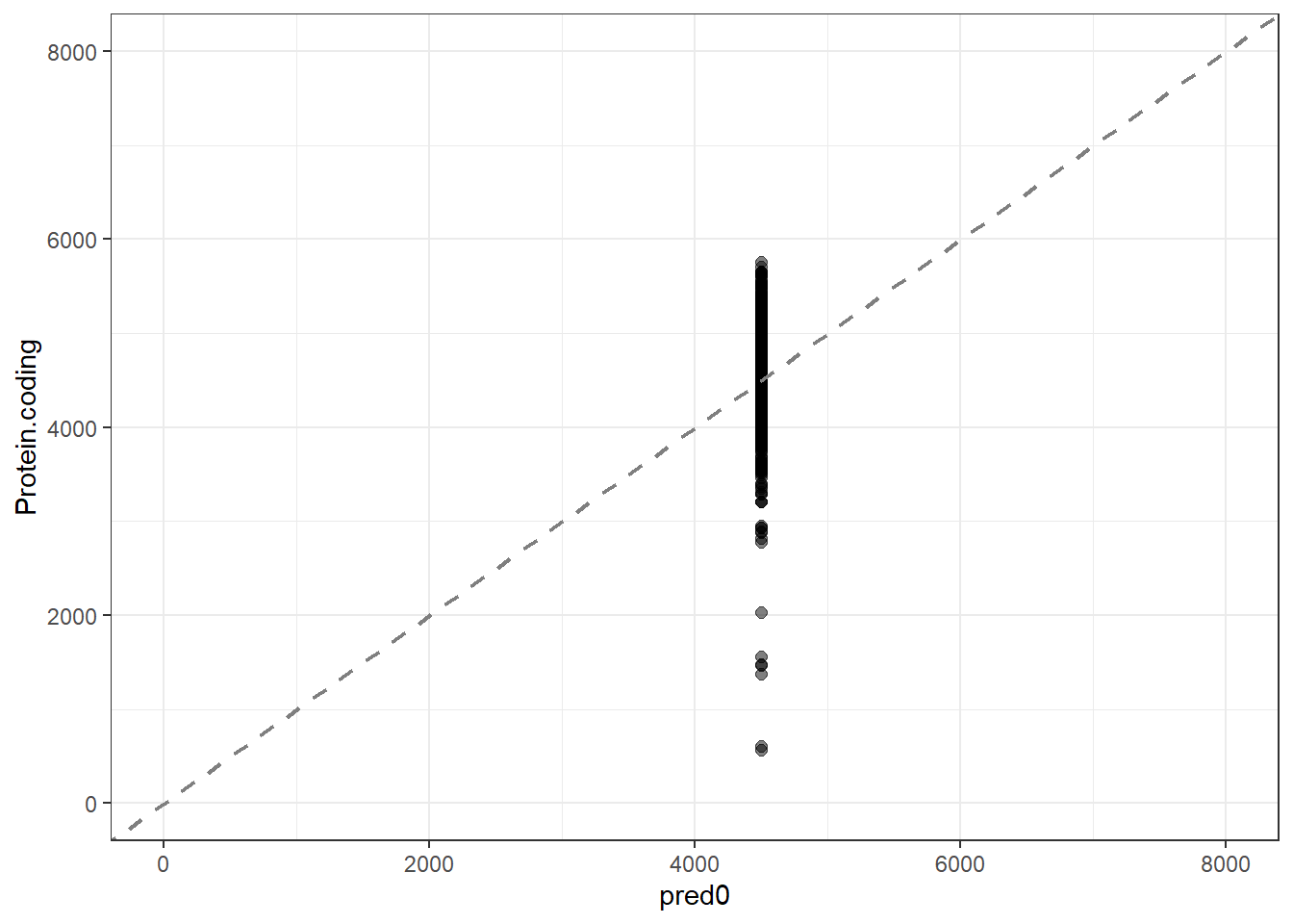
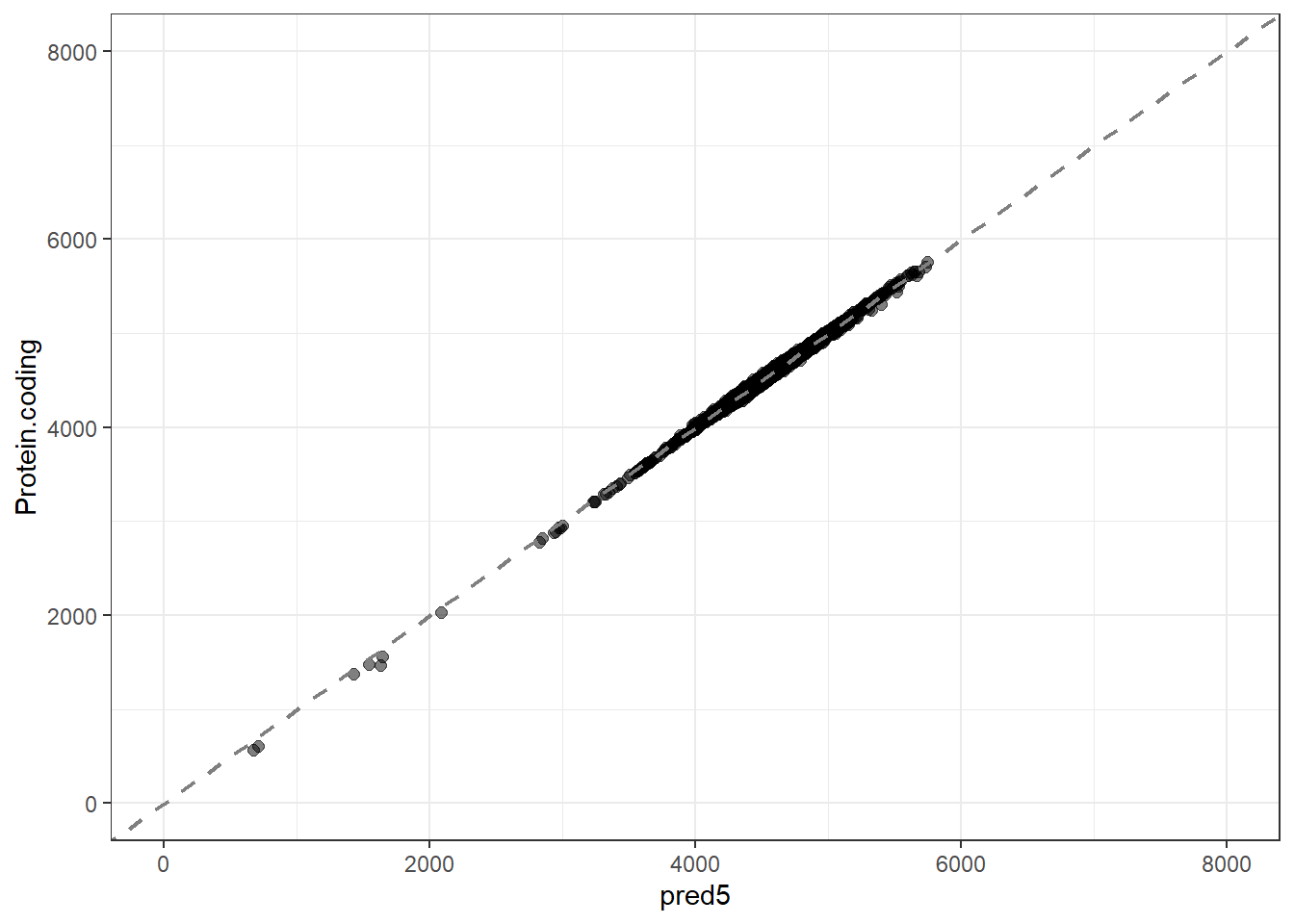
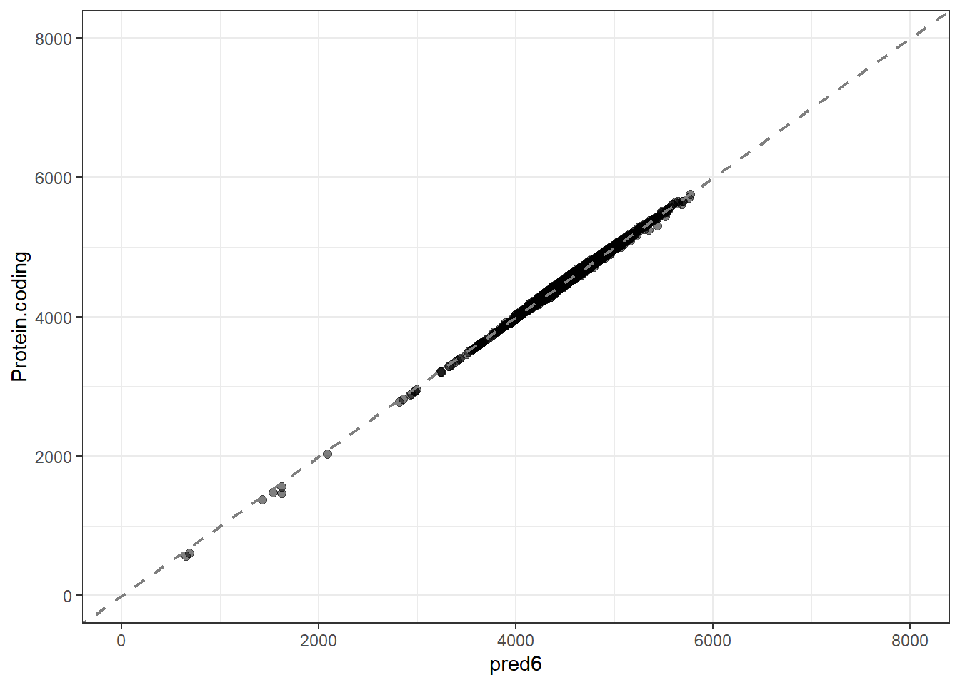
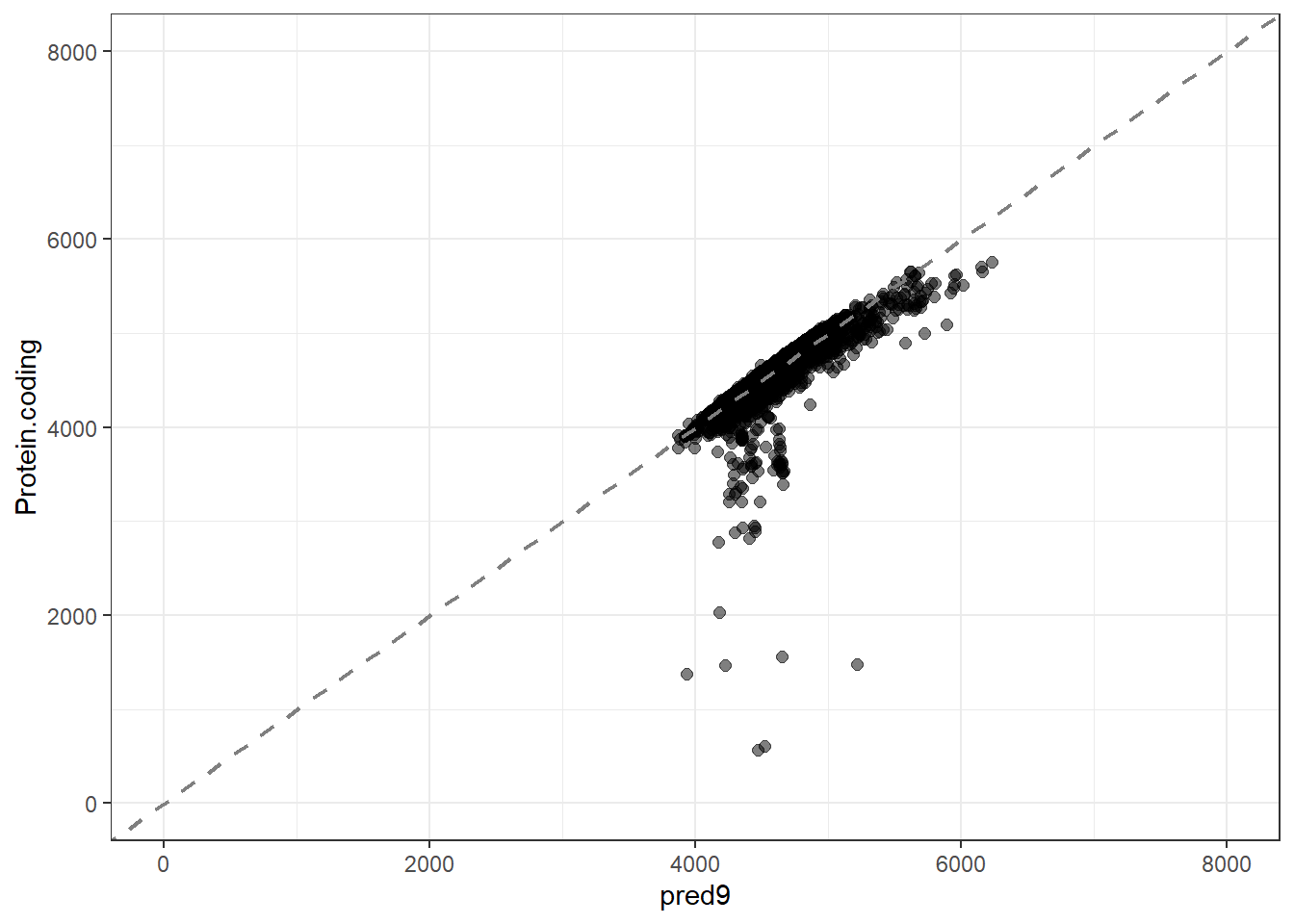
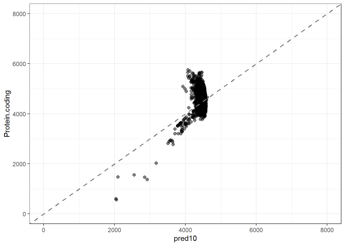
    pred0 = predict(lm_null, new_data = genomes1, type = "numeric")$.pred,
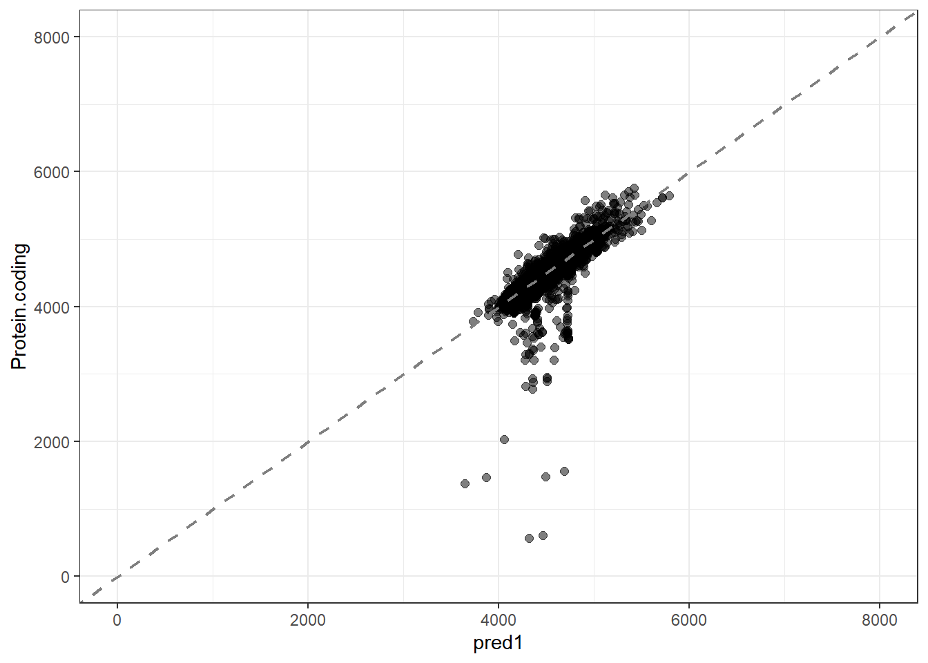
    pred1 = predict(lm_fit1, new_data = genomes1, type = "numeric")$.pred,
    pred2 = predict(lm_fit2, new_data = genomes1, type = "numeric")$.pred,
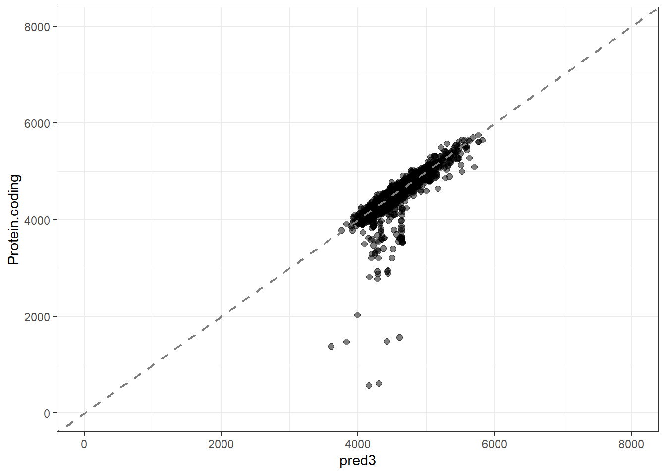
    pred3 = predict(lm_fit3, new_data = genomes1, type = "numeric")$.pred,
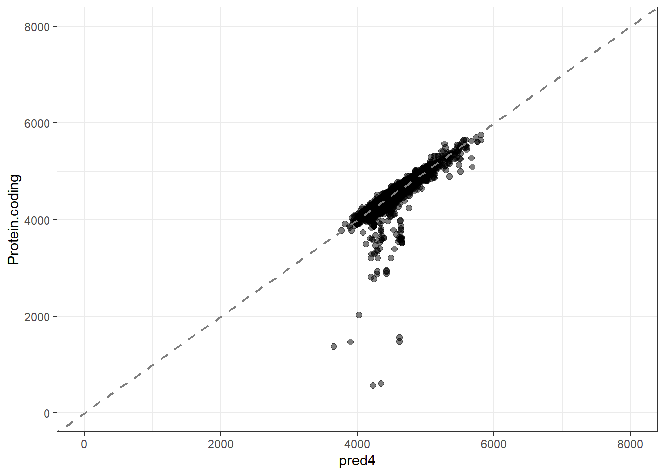
    pred4 = predict(lm_fit4, new_data = genomes1, type = "numeric")$.pred,
    pred5 = predict(lm_fit5, new_data = genomes1, type = "numeric")$.pred,
    pred6 = predict(lm_fit6, new_data = genomes1, type = "numeric")$.pred,
    pred7 = predict(lm_fit7, new_data = genomes1, type = "numeric")$.pred,
    pred8 = predict(lm_fit8, new_data = genomes1, type = "numeric")$.pred,
    pred9 = predict(lm_fit9, new_data = genomes1, type = "numeric")$.pred,
    pred10 = predict(lm_fit10, new_data = genomes1, type = "numeric")$.pred
  ) %>%
    mutate(
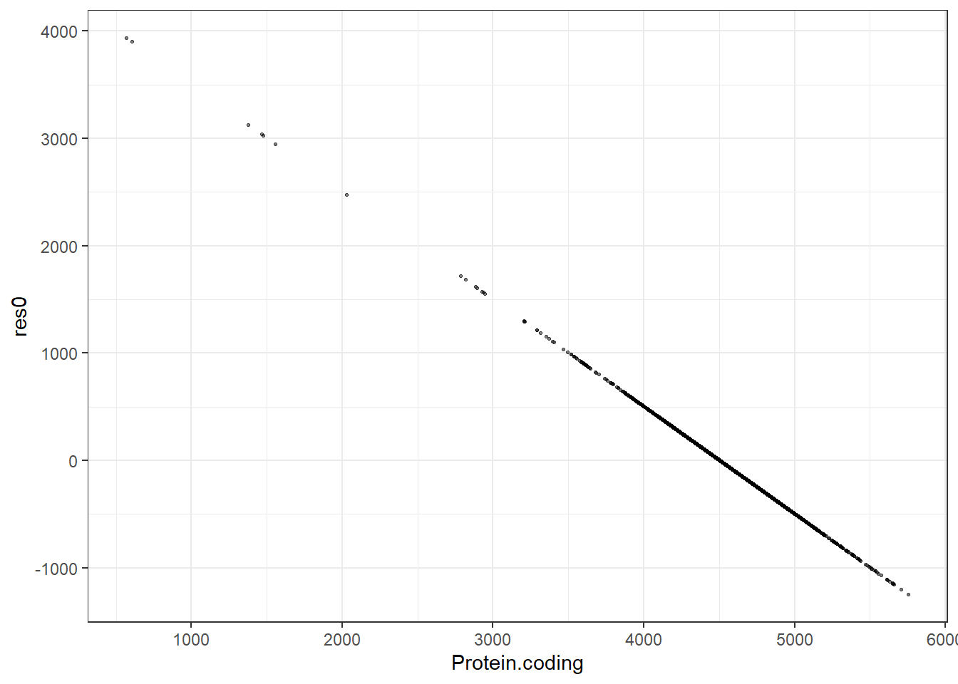
    res0 = pred0 - Protein.coding,
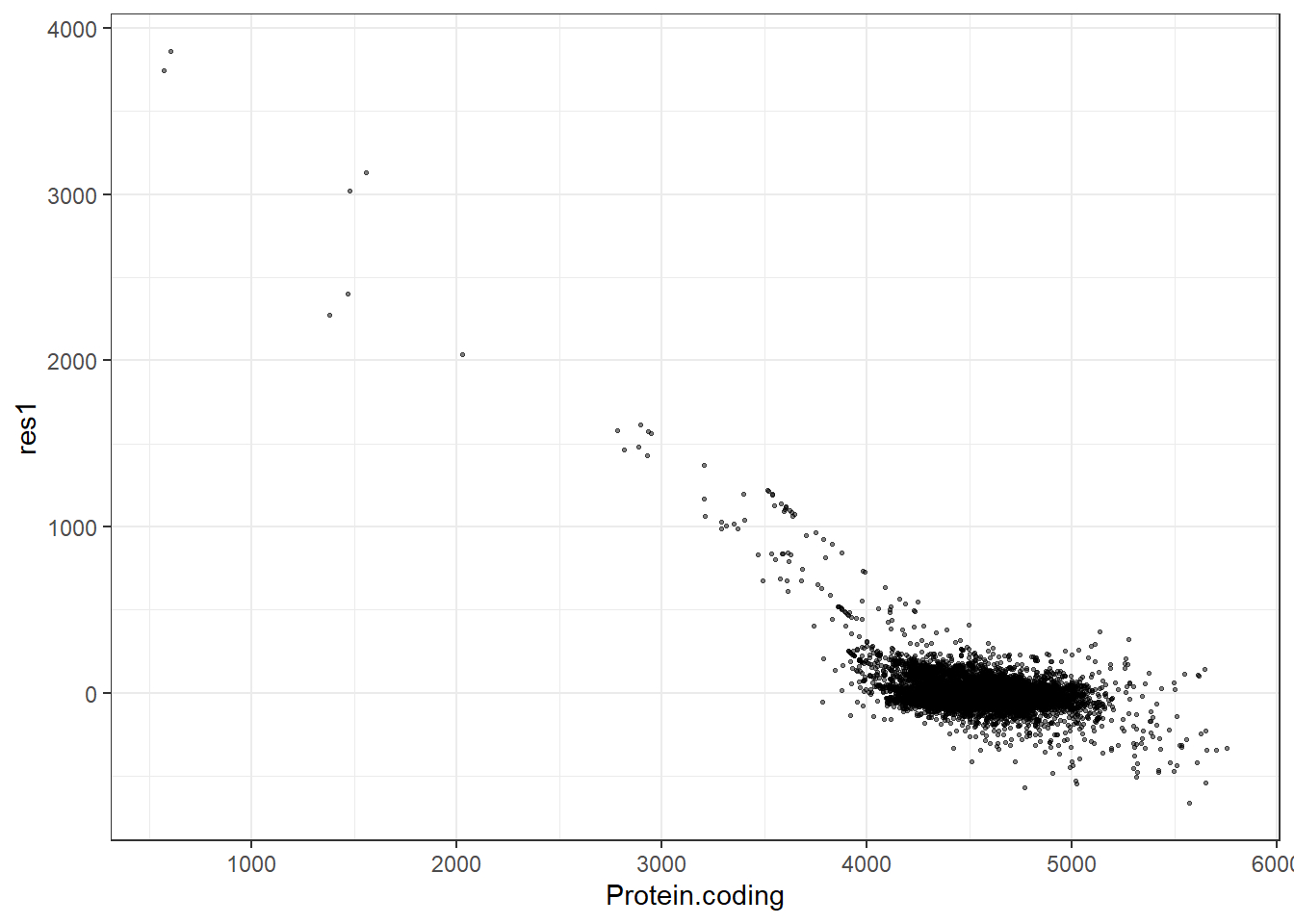
    res1 = pred1 - Protein.coding,
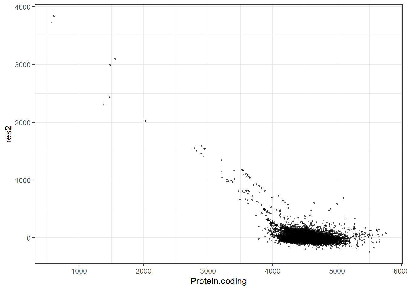
    res2 = pred2 - Protein.coding,
    res3 = pred3 - Protein.coding,
    res4 = pred4 - Protein.coding,
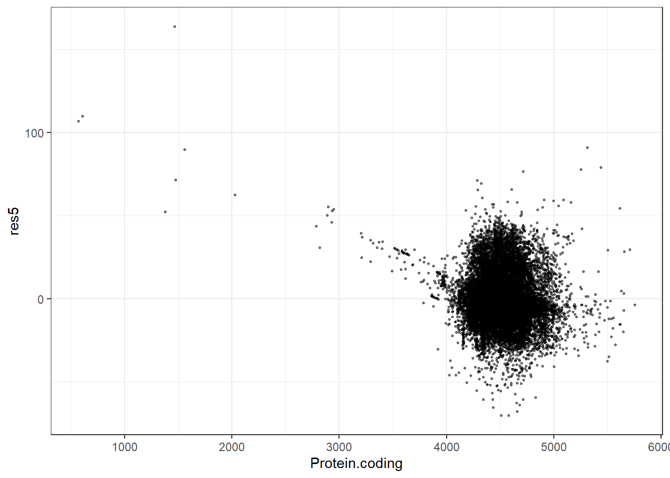
    res5 = pred5 - Protein.coding,
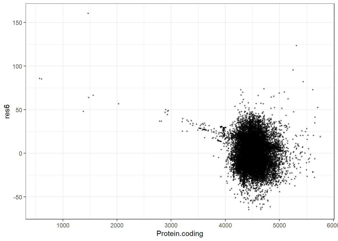
    res6 = pred6 - Protein.coding,
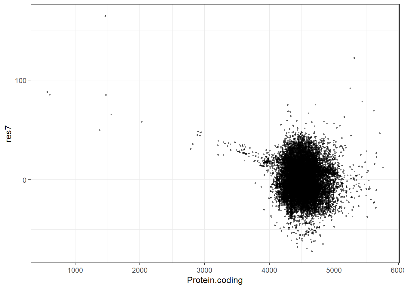
    res7 = pred7 - Protein.coding,
    res8 = pred8 - Protein.coding,
    res9 = pred9 - Protein.coding,
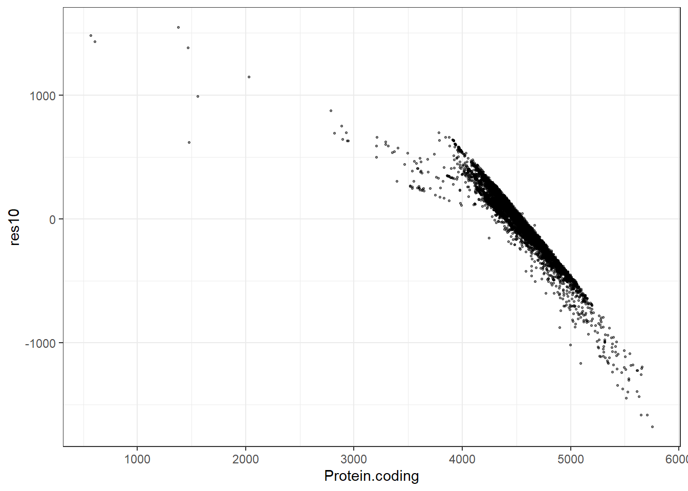
    res10 = pred10 - Protein.coding
  )

# Plotting predicted vs actual

ggplot(genomes1, aes(y = Protein.coding, x = pred0)) +
    geom_point(size = 2, alpha = 0.5) +
    geom_abline(slope = 1, intercept = 0, color = "gray50", linewidth = 0.8, linetype = "dashed") +
    lims(x = c(0, 8000), y = c(0, 8000)) +
    theme_bw()

ggplot(genomes1, aes(y = Protein.coding, x = pred1)) +
    geom_point(size = 2, alpha = 0.5) +
    geom_abline(slope = 1, intercept = 0, color = "gray50", linewidth = 0.8, linetype = "dashed") +
    lims(x = c(0, 8000), y = c(0, 8000)) +
    theme_bw()

ggplot(genomes1, aes(y = Protein.coding, x = pred2)) +
    geom_point(size = 2, alpha = 0.5) +
    geom_abline(slope = 1, intercept = 0, color = "gray50", linewidth = 0.8, linetype = "dashed") +
    lims(x = c(0, 8000), y = c(0, 8000)) +
    theme_bw()

ggplot(genomes1, aes(y = Protein.coding, x = pred3)) +
    geom_point(size = 2, alpha = 0.5) +
    geom_abline(slope = 1, intercept = 0, color = "gray50", linewidth = 0.8, linetype = "dashed") +
    lims(x = c(0, 8000), y = c(0, 8000)) +
    theme_bw()

ggplot(genomes1, aes(y = Protein.coding, x = pred4)) +
    geom_point(size = 2, alpha = 0.5) +
    geom_abline(slope = 1, intercept = 0, color = "gray50", linewidth = 0.8, linetype = "dashed") +
    lims(x = c(0, 8000), y = c(0, 8000)) +
    theme_bw()

ggplot(genomes1, aes(y = Protein.coding, x = pred5)) +
    geom_point(size = 2, alpha = 0.5) +
    geom_abline(slope = 1, intercept = 0, color = "gray50", linewidth = 0.8, linetype = "dashed") +
    lims(x = c(0, 8000), y = c(0, 8000)) +
    theme_bw()

ggplot(genomes1, aes(y = Protein.coding, x = pred6)) +
    geom_point(size = 2, alpha = 0.5) +
    geom_abline(slope = 1, intercept = 0, color = "gray50", linewidth = 0.8, linetype = "dashed") +
    lims(x = c(0, 8000), y = c(0, 8000)) +
    theme_bw()

ggplot(genomes1, aes(y = Protein.coding, x = pred7)) +
    geom_point(size = 2, alpha = 0.5) +
    geom_abline(slope = 1, intercept = 0, color = "gray50", linewidth = 0.8, linetype = "dashed") +
    lims(x = c(0, 8000), y = c(0, 8000)) +
    theme_bw()

ggplot(genomes1, aes(y = Protein.coding, x = pred8)) +
    geom_point(size = 2, alpha = 0.5) +
    geom_abline(slope = 1, intercept = 0, color = "gray50", linewidth = 0.8, linetype = "dashed") +
    lims(x = c(0, 8000), y = c(0, 8000)) +
    theme_bw()

ggplot(genomes1, aes(y = Protein.coding, x = pred9)) +
    geom_point(size = 2, alpha = 0.5) +
    geom_abline(slope = 1, intercept = 0, color = "gray50", linewidth = 0.8, linetype = "dashed") +
    lims(x = c(0, 8000), y = c(0, 8000)) +
    theme_bw()

ggplot(genomes1, aes(y = Protein.coding, x = pred10)) +
    geom_point(size = 2, alpha = 0.5) +
    geom_abline(slope = 1, intercept = 0, color = "gray50", linewidth = 0.8, linetype = "dashed") +
    lims(x = c(0, 8000), y = c(0, 8000)) +
    theme_bw()

# Plotting residuals

ggplot(genomes1, aes(x = Protein.coding, y = res0)) +
    geom_point(size = 0.5, alpha = 0.5) +
    theme_bw()

ggplot(genomes1, aes(x = Protein.coding, y = res1)) +
    geom_point(size = 0.5, alpha = 0.5) +
    theme_bw()

ggplot(genomes1, aes(x = Protein.coding, y = res2)) +
    geom_point(size = 0.5, alpha = 0.5) +
    theme_bw()

ggplot(genomes1, aes(x = Protein.coding, y = res3)) +
    geom_point(size = 0.5, alpha = 0.5) +
    theme_bw()

ggplot(genomes1, aes(x = Protein.coding, y = res4)) +
    geom_point(size = 0.5, alpha = 0.5) +
    theme_bw()

ggplot(genomes1, aes(x = Protein.coding,  y= res5)) +
    geom_point(size = 0.5, alpha = 0.5) +
    theme_bw()

ggplot(genomes1, aes(x = Protein.coding,  y= res6)) +
    geom_point(size = 0.5, alpha = 0.5) +
    theme_bw()

ggplot(genomes1, aes(x = Protein.coding,  y= res7)) +
    geom_point(size = 0.5, alpha = 0.5) +
    theme_bw()

ggplot(genomes1, aes(x = Protein.coding,  y= res8)) +
    geom_point(size = 0.5, alpha = 0.5) +
    theme_bw()

ggplot(genomes1, aes(x = Protein.coding,  y= res9)) +
    geom_point(size = 0.5, alpha = 0.5) +
    theme_bw()

ggplot(genomes1, aes(x = Protein.coding,  y= res10)) +
    geom_point(size = 0.5, alpha = 0.5) +
    theme_bw()

AIC(extract_fit_engine(lm_null))

[1] 279299.1

AIC(extract_fit_engine(lm_fit1))

[1] 249583.7

AIC(extract_fit_engine(lm_fit2))

[1] 247457.7

AIC(extract_fit_engine(lm_fit3))

[1] 245720.7

AIC(extract_fit_engine(lm_fit4))

[1] 245479.1

AIC(extract_fit_engine(lm_fit5))

[1] 170202.9

AIC(extract_fit_engine(lm_fit6))

[1] 173461.1

AIC(extract_fit_engine(lm_fit7))

[1] 173648.8

AIC(extract_fit_engine(lm_fit8))

[1] 247042.8

AIC(extract_fit_engine(lm_fit9))

[1] 249564.3

AIC(extract_fit_engine(lm_fit10))

[1] 277147.8

# Create a NAMED list 
model_list <- list(
  null  = lm_null,
  fit1  = lm_fit1, fit2  = lm_fit2, fit3  = lm_fit3,
  fit4  = lm_fit4, fit5  = lm_fit5, fit6  = lm_fit6,
  fit7  = lm_fit7, fit8  = lm_fit8, fit9  = lm_fit9,
  fit10 = lm_fit10
)

# Extract AIC from list and create a tibble
AIC_df <- map_dfr(model_list, ~{
  engine <- extract_fit_engine(.x)
  tibble(AIC = AIC(engine))
}, .id = "model_id")

# Plot 
AIC_df %>%
  arrange(desc(AIC)) %>%  
  mutate(model_id = factor(model_id, levels = model_id)) %>%  
  ggplot(aes(x = model_id, y = AIC)) +
  geom_col() +
  theme_bw() +
  labs(x = "Model", y = "AIC")