RANDOM FOREST APPROACH

I wanted to go for a different approach for something that does not have a linear relationship. For that I wanted to approach to predict AMR based on metadata like serotype, source type, and even month of the year.

library(lubridate)

Attaching package: 'lubridate'

The following objects are masked from 'package:base':

    date, intersect, setdiff, union

library(tidyverse)

── Attaching core tidyverse packages ──────────────────────── tidyverse 2.0.0 ──
✔ dplyr   1.1.4     ✔ readr   2.2.0
✔ forcats 1.0.1     ✔ stringr 1.6.0
✔ ggplot2 3.5.2     ✔ tibble  3.2.1
✔ purrr   1.2.1     ✔ tidyr   1.3.2

── Conflicts ────────────────────────────────────────── tidyverse_conflicts() ──
✖ dplyr::filter() masks stats::filter()
✖ dplyr::lag()    masks stats::lag()
ℹ Use the conflicted package (<http://conflicted.r-lib.org/>) to force all conflicts to become errors

library(tidymodels)

── Attaching packages ────────────────────────────────────── tidymodels 1.4.1 ──
✔ broom        1.0.12     ✔ rsample      1.3.2 
✔ dials        1.4.2      ✔ tailor       0.1.0 
✔ infer        1.1.0      ✔ tune         2.0.1 
✔ modeldata    1.5.1      ✔ workflows    1.3.0 
✔ parsnip      1.4.1      ✔ workflowsets 1.1.1 
✔ recipes      1.3.1      ✔ yardstick    1.3.2 
── Conflicts ───────────────────────────────────────── tidymodels_conflicts() ──
✖ scales::discard() masks purrr::discard()
✖ dplyr::filter()   masks stats::filter()
✖ recipes::fixed()  masks stringr::fixed()
✖ dplyr::lag()      masks stats::lag()
✖ yardstick::spec() masks readr::spec()
✖ recipes::step()   masks stats::step()

library(here)

here() starts at C:/Users/marco/Documents/marcoreina-MADA-project

library(vip)

Attaching package: 'vip'

The following object is masked from 'package:utils':

    vi

library(gt)

# Read data
amr_long_rf <- read_csv(here("data/processed-data/amr_long.csv"))

Rows: 688980 Columns: 10
── Column specification ────────────────────────────────────────────────────────
Delimiter: ","
chr  (8): Isolation.source, Source.type, BioSample, antigen_formula, serotyp...
dbl  (1): year
dttm (1): Create.date

ℹ Use `spec()` to retrieve the full column specification for this data.
ℹ Specify the column types or set `show_col_types = FALSE` to quiet this message.

amr_long_rf <- amr_long_rf %>%
  mutate(AMR_class_strict = if_else(AMR_status == "COMPLETE", AMR_class, "NO AMR"))

amr_wide_rf <- amr_long_rf %>%
  select(Create.date, BioSample, AMR_class_strict, serotype, Source.type) %>%
  distinct(BioSample, AMR_class_strict, .keep_all = TRUE) %>%
  mutate(present = 1) %>%
  pivot_wider(
    id_cols = c(Create.date, BioSample, serotype, Source.type),
    names_from = AMR_class_strict,
    values_from = present,
    values_fill = 0
  ) 

amr_wide_rf$`Efflux Pump` = NULL
amr_wide_rf$`NO AMR` = NULL 

amr_wide_rf <- amr_wide_rf %>%
  mutate(
    sample_year = as.factor(year(Create.date)),
    sample_month = month(Create.date, label = TRUE),
    total_amr_classes = rowSums(across(c("Aminoglycoside", "Fosfomycin","Beta_lactam", "Gentamicin", "Trimethoprim", "Quinolone", "Phenicol", "Colistin", "Macrolide", "Bleomycin", "Tetracycline", "Sulfonamide", "Lincosamide"))),
    amr_prevalence = if_else(total_amr_classes == 0, 0, 1),
    mdr_prevalence = if_else(total_amr_classes <= 3, 0, 1)
  )

# Get the total number of isolates
totaln_isolates <- nrow(amr_wide_rf)

top_20_serovars <- amr_wide_rf %>%
    group_by(serotype) %>%
    summarise(
        n = n(),
        amr_positive = sum(amr_prevalence, na.rm = TRUE),
        mdr_positive = sum(mdr_prevalence, na.rm = TRUE),
        .groups = "drop"
    ) %>%
    mutate(
        serovar_pct = round(n / totaln_isolates * 100, 1),
        amr_pct = round(amr_positive / totaln_isolates * 100, 1),
        mdr_pct = round(mdr_positive / totaln_isolates * 100, 1)
    ) %>%
     slice_max(n, n = 20, with_ties = FALSE) %>%
         arrange(desc(amr_positive)) 


#Creating list with top serovars
top_20 <- c("I 4,[5],12:i:-", "Infantis", "Typhimurium", "Newport", "Agona", "Kentucky", "Enteritidis", "Anatum",     "Saintpaul", "Braenderup", "Muenchen", "Sandiego", "Javiana", "Montevideo", "Oranienburg", "Thompson", "Mississippi", "Bareilly", "Poona", "Rubislaw")

# Creating the new column to  "Other" for serovars that are not in the top 20
amr_wide_rf <- amr_wide_rf %>%
  mutate(top_20 = if_else(serotype %in% top_20, serotype, "Other"))

# Set seed
rngseed <- 1234
set.seed(rngseed)

amr_wide_rf <- amr_wide_rf %>%
  mutate(amr_prevalence = factor(amr_prevalence, levels = c(1, 0)),
          Tetracycline = factor(Tetracycline, levels = c(1, 0)),           
          Aminoglycoside = factor(Aminoglycoside, levels = c(1, 0)),  
          Sulfonamide = factor(Sulfonamide, levels = c(1, 0)),  
          Beta_lactam = factor(Beta_lactam, levels = c(1, 0)),  
          Phenicol = factor(Phenicol, levels = c(1, 0)),   
  )

amr_wide_rf <- amr_wide_rf %>%
  mutate()

set.seed(rngseed)

split <- initial_split(amr_wide_rf, prop = 0.75, strata = amr_prevalence)

train_data <- training(split)
test_data  <- testing(split)

rf_spec <- rand_forest(
  mode = "classification",
  trees = 500,
  mtry = floor(sqrt(ncol(train_data) - 1)),
  min_n = 5
) %>%
  set_engine("ranger", seed = rngseed, importance = "permutation")

rf_fit_tet <- rf_spec %>%
  fit(Tetracycline ~ Source.type + top_20 + sample_month, data = train_data)

Warning: ! 5 columns were requested but there were 3 predictors in the data.
ℹ 3 predictors will be used.

rf_fit_tet 

parsnip model object

Ranger result

Call:
 ranger::ranger(x = maybe_data_frame(x), y = y, mtry = min_cols(~floor(sqrt(ncol(train_data) -      1)), x), num.trees = ~500, min.node.size = min_rows(~5, x),      seed = ~rngseed, importance = ~"permutation", num.threads = 1,      verbose = FALSE, probability = TRUE) 

Type:                             Probability estimation 
Number of trees:                  500 
Sample size:                      184328 
Number of independent variables:  3 
Mtry:                             3 
Target node size:                 5 
Variable importance mode:         permutation 
Splitrule:                        gini 
OOB prediction error (Brier s.):  0.07110536 

test_pred_tet <- test_data %>%
  bind_cols(
    predict(rf_fit_tet, new_data = test_data),                
    predict(rf_fit_tet, new_data = test_data, type = "prob")   
  )

conf_mat(test_pred_tet, truth = Tetracycline, estimate = .pred_class)

          Truth
Prediction     1     0
         1  2374  1323
         0  4339 53407

sens(test_pred_tet, truth = Tetracycline, estimate = .pred_class)

# A tibble: 1 × 3
  .metric .estimator .estimate
  <chr>   <chr>          <dbl>
1 sens    binary         0.354

spec(test_pred_tet, truth = Tetracycline, estimate = .pred_class)

# A tibble: 1 × 3
  .metric .estimator .estimate
  <chr>   <chr>          <dbl>
1 spec    binary         0.976

accuracy(test_pred_tet, truth = Tetracycline, estimate = .pred_class)

# A tibble: 1 × 3
  .metric  .estimator .estimate
  <chr>    <chr>          <dbl>
1 accuracy binary         0.908

precision(test_pred_tet, truth = Tetracycline, estimate = .pred_class)

# A tibble: 1 × 3
  .metric   .estimator .estimate
  <chr>     <chr>          <dbl>
1 precision binary         0.642

f_meas(test_pred_tet, truth = Tetracycline, estimate = .pred_class) 

# A tibble: 1 × 3
  .metric .estimator .estimate
  <chr>   <chr>          <dbl>
1 f_meas  binary         0.456

roc_curve(test_pred_tet, truth = Tetracycline, .pred_1) %>%
  autoplot()

roc_auc(test_pred_tet, truth = Tetracycline, .pred_1)

# A tibble: 1 × 3
  .metric .estimator .estimate
  <chr>   <chr>          <dbl>
1 roc_auc binary         0.837

ggplot(test_pred_tet, aes(x = .pred_1, fill = Tetracycline)) +
  geom_density(alpha = 0.5) +
  theme_bw()

# Extract and plot
rf_fit_tet %>%
  extract_fit_engine() %>%
  vip(num_features = 10) +
  theme_bw() +
  labs(title = "Variable Importance for Tetracycline Resistance Prediction")

set.seed(rngseed)

rf_fit_ami <- rf_spec %>%
  fit(Aminoglycoside ~ Source.type + top_20 + sample_month, data = train_data)

Warning: ! 5 columns were requested but there were 3 predictors in the data.
ℹ 3 predictors will be used.

rf_fit_ami

parsnip model object

Ranger result

Call:
 ranger::ranger(x = maybe_data_frame(x), y = y, mtry = min_cols(~floor(sqrt(ncol(train_data) -      1)), x), num.trees = ~500, min.node.size = min_rows(~5, x),      seed = ~rngseed, importance = ~"permutation", num.threads = 1,      verbose = FALSE, probability = TRUE) 

Type:                             Probability estimation 
Number of trees:                  500 
Sample size:                      184328 
Number of independent variables:  3 
Mtry:                             3 
Target node size:                 5 
Variable importance mode:         permutation 
Splitrule:                        gini 
OOB prediction error (Brier s.):  0.06655703 

test_pred_ami <- test_data %>%
  bind_cols(
    predict(rf_fit_ami, new_data = test_data),                
    predict(rf_fit_ami, new_data = test_data, type = "prob")   
  )

conf_mat(test_pred_ami, truth = Aminoglycoside, estimate = .pred_class)

          Truth
Prediction     1     0
         1  2067  1300
         0  3960 54116

sens(test_pred_ami, truth = Aminoglycoside, estimate = .pred_class)

# A tibble: 1 × 3
  .metric .estimator .estimate
  <chr>   <chr>          <dbl>
1 sens    binary         0.343

spec(test_pred_ami, truth = Aminoglycoside, estimate = .pred_class)

# A tibble: 1 × 3
  .metric .estimator .estimate
  <chr>   <chr>          <dbl>
1 spec    binary         0.977

accuracy(test_pred_ami, truth = Aminoglycoside, estimate = .pred_class)

# A tibble: 1 × 3
  .metric  .estimator .estimate
  <chr>    <chr>          <dbl>
1 accuracy binary         0.914

precision(test_pred_ami, truth = Aminoglycoside, estimate = .pred_class)

# A tibble: 1 × 3
  .metric   .estimator .estimate
  <chr>     <chr>          <dbl>
1 precision binary         0.614

f_meas(test_pred_ami, truth = Aminoglycoside, estimate = .pred_class) 

# A tibble: 1 × 3
  .metric .estimator .estimate
  <chr>   <chr>          <dbl>
1 f_meas  binary         0.440

roc_curve(test_pred_ami, truth = Aminoglycoside, .pred_1) %>%
  autoplot()

roc_auc(test_pred_ami, truth = Aminoglycoside, .pred_1)

# A tibble: 1 × 3
  .metric .estimator .estimate
  <chr>   <chr>          <dbl>
1 roc_auc binary         0.847

ggplot(test_pred_ami, aes(x = .pred_1, fill = Aminoglycoside)) +
  geom_density(alpha = 0.5) +
  theme_bw()

# Extract and plot
rf_fit_ami %>%
  extract_fit_engine() %>%
  vip(num_features = 10) +
  theme_bw() +
  labs(title = "Variable Importance for Aminoglycoside Resistance Prediction")

set.seed(rngseed)
rf_fit_sul <- rf_spec %>%
  fit(Sulfonamide ~ Source.type + top_20 + sample_month, data = train_data)

Warning: ! 5 columns were requested but there were 3 predictors in the data.
ℹ 3 predictors will be used.

rf_fit_sul

parsnip model object

Ranger result

Call:
 ranger::ranger(x = maybe_data_frame(x), y = y, mtry = min_cols(~floor(sqrt(ncol(train_data) -      1)), x), num.trees = ~500, min.node.size = min_rows(~5, x),      seed = ~rngseed, importance = ~"permutation", num.threads = 1,      verbose = FALSE, probability = TRUE) 

Type:                             Probability estimation 
Number of trees:                  500 
Sample size:                      184328 
Number of independent variables:  3 
Mtry:                             3 
Target node size:                 5 
Variable importance mode:         permutation 
Splitrule:                        gini 
OOB prediction error (Brier s.):  0.05868647 

test_pred_sul <- test_data %>%
  bind_cols(
    predict(rf_fit_sul, new_data = test_data),                 
    predict(rf_fit_sul, new_data = test_data, type = "prob")   
  )

conf_mat(test_pred_sul, truth = Sulfonamide, estimate = .pred_class)

          Truth
Prediction     1     0
         1  1728  1280
         0  3421 55014

sens(test_pred_sul, truth = Sulfonamide, estimate = .pred_class)

# A tibble: 1 × 3
  .metric .estimator .estimate
  <chr>   <chr>          <dbl>
1 sens    binary         0.336

spec(test_pred_sul, truth = Sulfonamide, estimate = .pred_class)

# A tibble: 1 × 3
  .metric .estimator .estimate
  <chr>   <chr>          <dbl>
1 spec    binary         0.977

accuracy(test_pred_sul, truth = Sulfonamide, estimate = .pred_class)

# A tibble: 1 × 3
  .metric  .estimator .estimate
  <chr>    <chr>          <dbl>
1 accuracy binary         0.923

precision(test_pred_sul, truth = Sulfonamide, estimate = .pred_class)

# A tibble: 1 × 3
  .metric   .estimator .estimate
  <chr>     <chr>          <dbl>
1 precision binary         0.574

f_meas(test_pred_sul, truth = Sulfonamide, estimate = .pred_class) 

# A tibble: 1 × 3
  .metric .estimator .estimate
  <chr>   <chr>          <dbl>
1 f_meas  binary         0.424

roc_curve(test_pred_sul, truth = Sulfonamide, .pred_1) %>%
  autoplot()

roc_auc(test_pred_sul, truth = Sulfonamide, .pred_1)

# A tibble: 1 × 3
  .metric .estimator .estimate
  <chr>   <chr>          <dbl>
1 roc_auc binary         0.850

ggplot(test_pred_sul, aes(x = .pred_1, fill = Sulfonamide)) +
  geom_density(alpha = 0.5) +
  theme_bw()

# Extract and plot
rf_fit_sul %>%
  extract_fit_engine() %>%
  vip(num_features = 10) +
  theme_bw() +
  labs(title = "Variable Importance for Sulfonamide Resistance Prediction")

set.seed(rngseed)

rf_fit_bet <- rf_spec %>%
  fit(Beta_lactam ~ Source.type + top_20 + sample_month, data = train_data)

Warning: ! 5 columns were requested but there were 3 predictors in the data.
ℹ 3 predictors will be used.

rf_fit_bet

parsnip model object

Ranger result

Call:
 ranger::ranger(x = maybe_data_frame(x), y = y, mtry = min_cols(~floor(sqrt(ncol(train_data) -      1)), x), num.trees = ~500, min.node.size = min_rows(~5, x),      seed = ~rngseed, importance = ~"permutation", num.threads = 1,      verbose = FALSE, probability = TRUE) 

Type:                             Probability estimation 
Number of trees:                  500 
Sample size:                      184328 
Number of independent variables:  3 
Mtry:                             3 
Target node size:                 5 
Variable importance mode:         permutation 
Splitrule:                        gini 
OOB prediction error (Brier s.):  0.05363896 

test_pred_bet <- test_data %>%
  bind_cols(
    predict(rf_fit_bet, new_data = test_data),                 
    predict(rf_fit_bet, new_data = test_data, type = "prob")   
  )

conf_mat(test_pred_bet, truth = Beta_lactam, estimate = .pred_class)

          Truth
Prediction     1     0
         1  1263  1004
         0  3111 56065

sens(test_pred_bet, truth = Beta_lactam, estimate = .pred_class)

# A tibble: 1 × 3
  .metric .estimator .estimate
  <chr>   <chr>          <dbl>
1 sens    binary         0.289

spec(test_pred_bet, truth = Beta_lactam, estimate = .pred_class)

# A tibble: 1 × 3
  .metric .estimator .estimate
  <chr>   <chr>          <dbl>
1 spec    binary         0.982

accuracy(test_pred_bet, truth = Beta_lactam, estimate = .pred_class)

# A tibble: 1 × 3
  .metric  .estimator .estimate
  <chr>    <chr>          <dbl>
1 accuracy binary         0.933

precision(test_pred_bet, truth = Beta_lactam, estimate = .pred_class)

# A tibble: 1 × 3
  .metric   .estimator .estimate
  <chr>     <chr>          <dbl>
1 precision binary         0.557

f_meas(test_pred_bet, truth = Beta_lactam, estimate = .pred_class) 

# A tibble: 1 × 3
  .metric .estimator .estimate
  <chr>   <chr>          <dbl>
1 f_meas  binary         0.380

roc_curve(test_pred_bet, truth = Beta_lactam, .pred_1) %>%
  autoplot()

roc_auc(test_pred_bet, truth = Beta_lactam, .pred_1)

# A tibble: 1 × 3
  .metric .estimator .estimate
  <chr>   <chr>          <dbl>
1 roc_auc binary         0.812

ggplot(test_pred_bet, aes(x = .pred_1, fill = Beta_lactam)) +
  geom_density(alpha = 0.5) +
  theme_bw()

# Extract and plot
rf_fit_bet %>%
  extract_fit_engine() %>%
  vip(num_features = 10) +
  theme_bw() +
  labs(title = "Variable Importance for Beta lactams Prediction")

set.seed(rngseed)

rf_fit_phe <- rf_spec %>%
  fit(Phenicol ~ Source.type + top_20 + sample_month, data = train_data)

Warning: ! 5 columns were requested but there were 3 predictors in the data.
ℹ 3 predictors will be used.

rf_fit_phe

parsnip model object

Ranger result

Call:
 ranger::ranger(x = maybe_data_frame(x), y = y, mtry = min_cols(~floor(sqrt(ncol(train_data) -      1)), x), num.trees = ~500, min.node.size = min_rows(~5, x),      seed = ~rngseed, importance = ~"permutation", num.threads = 1,      verbose = FALSE, probability = TRUE) 

Type:                             Probability estimation 
Number of trees:                  500 
Sample size:                      184328 
Number of independent variables:  3 
Mtry:                             3 
Target node size:                 5 
Variable importance mode:         permutation 
Splitrule:                        gini 
OOB prediction error (Brier s.):  0.03730023 

test_pred_phe <- test_data %>%
  bind_cols(
    predict(rf_fit_phe, new_data = test_data),                 
    predict(rf_fit_phe, new_data = test_data, type = "prob")   
  )

conf_mat(test_pred_phe, truth = Phenicol, estimate = .pred_class)

          Truth
Prediction     1     0
         1     4     5
         0  2512 58922

sens(test_pred_phe, truth = Phenicol, estimate = .pred_class)

# A tibble: 1 × 3
  .metric .estimator .estimate
  <chr>   <chr>          <dbl>
1 sens    binary       0.00159

spec(test_pred_phe, truth = Phenicol, estimate = .pred_class)

# A tibble: 1 × 3
  .metric .estimator .estimate
  <chr>   <chr>          <dbl>
1 spec    binary         1.000

accuracy(test_pred_phe, truth = Phenicol, estimate = .pred_class)

# A tibble: 1 × 3
  .metric  .estimator .estimate
  <chr>    <chr>          <dbl>
1 accuracy binary         0.959

precision(test_pred_phe, truth = Phenicol, estimate = .pred_class)

# A tibble: 1 × 3
  .metric   .estimator .estimate
  <chr>     <chr>          <dbl>
1 precision binary         0.444

f_meas(test_pred_phe, truth = Phenicol, estimate = .pred_class) 

# A tibble: 1 × 3
  .metric .estimator .estimate
  <chr>   <chr>          <dbl>
1 f_meas  binary       0.00317

roc_curve(test_pred_phe, truth = Phenicol, .pred_1) %>%
  autoplot()

roc_auc(test_pred_phe, truth = Phenicol, .pred_1)

# A tibble: 1 × 3
  .metric .estimator .estimate
  <chr>   <chr>          <dbl>
1 roc_auc binary         0.808

ggplot(test_pred_phe, aes(x = .pred_1, fill = Phenicol)) +
  geom_density(alpha = 0.5) +
  theme_bw()

# Extract and plot
rf_fit_phe %>%
  extract_fit_engine() %>%
  vip(num_features = 10) +
  theme_bw() +
  labs(title = "Variable Importance for Beta lactams Prediction")

set.seed(rngseed)

rf_fit_amr <- rf_spec %>%
  fit(amr_prevalence ~ Source.type + top_20 + sample_month, data = train_data)

Warning: ! 5 columns were requested but there were 3 predictors in the data.
ℹ 3 predictors will be used.

rf_fit_amr

parsnip model object

Ranger result

Call:
 ranger::ranger(x = maybe_data_frame(x), y = y, mtry = min_cols(~floor(sqrt(ncol(train_data) -      1)), x), num.trees = ~500, min.node.size = min_rows(~5, x),      seed = ~rngseed, importance = ~"permutation", num.threads = 1,      verbose = FALSE, probability = TRUE) 

Type:                             Probability estimation 
Number of trees:                  500 
Sample size:                      184328 
Number of independent variables:  3 
Mtry:                             3 
Target node size:                 5 
Variable importance mode:         permutation 
Splitrule:                        gini 
OOB prediction error (Brier s.):  0.09430651 

test_pred5 <- test_data %>%
  bind_cols(
    predict(rf_fit_amr, new_data = test_data),                 
    predict(rf_fit_amr, new_data = test_data, type = "prob")   
  )

conf_mat(test_pred5, truth = amr_prevalence, estimate = .pred_class)

          Truth
Prediction     1     0
         1  3391  1166
         0  6236 50650

sens(test_pred5, truth = amr_prevalence, estimate = .pred_class)

# A tibble: 1 × 3
  .metric .estimator .estimate
  <chr>   <chr>          <dbl>
1 sens    binary         0.352

spec(test_pred5, truth = amr_prevalence, estimate = .pred_class)

# A tibble: 1 × 3
  .metric .estimator .estimate
  <chr>   <chr>          <dbl>
1 spec    binary         0.977

accuracy(test_pred5, truth = amr_prevalence, estimate = .pred_class)

# A tibble: 1 × 3
  .metric  .estimator .estimate
  <chr>    <chr>          <dbl>
1 accuracy binary         0.880

precision(test_pred5, truth = amr_prevalence, estimate = .pred_class)

# A tibble: 1 × 3
  .metric   .estimator .estimate
  <chr>     <chr>          <dbl>
1 precision binary         0.744

f_meas(test_pred5, truth = amr_prevalence, estimate = .pred_class) 

# A tibble: 1 × 3
  .metric .estimator .estimate
  <chr>   <chr>          <dbl>
1 f_meas  binary         0.478

roc_curve(test_pred5, truth = amr_prevalence, .pred_1) %>%
  autoplot()

roc_auc(test_pred5, truth = amr_prevalence, .pred_1)

# A tibble: 1 × 3
  .metric .estimator .estimate
  <chr>   <chr>          <dbl>
1 roc_auc binary         0.825

ggplot(test_pred5, aes(x = .pred_1, fill = amr_prevalence)) +
  geom_density(alpha = 0.5) +
  theme_bw()

# Extract and plot
rf_fit_amr %>%
  extract_fit_engine() %>%
  vip(num_features = 10) +
  theme_bw() +
  labs(title = "Variable Importance for AMR Prediction")

# Create a function to extract metrics from each prediction object
get_metrics <- function(pred_df, truth_col, model_name) {
  list(
    sens(pred_df, truth = !!sym(truth_col), estimate = .pred_class),
    spec(pred_df, truth = !!sym(truth_col), estimate = .pred_class),
    accuracy(pred_df, truth = !!sym(truth_col), estimate = .pred_class),
    precision(pred_df, truth = !!sym(truth_col), estimate = .pred_class),
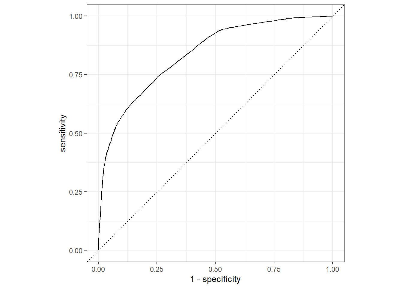
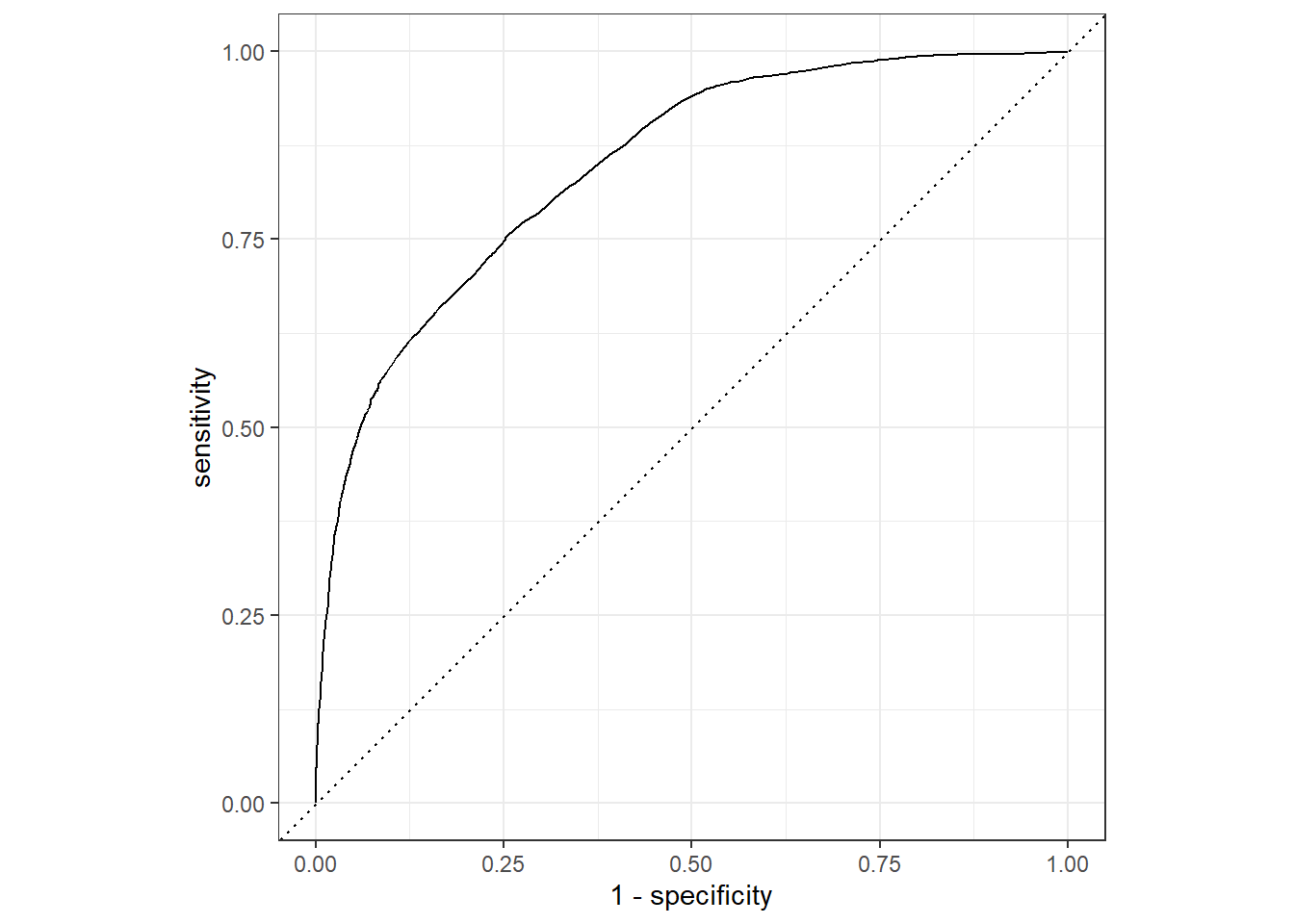
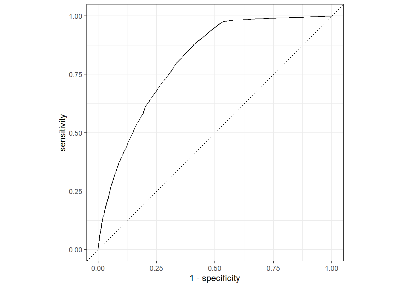
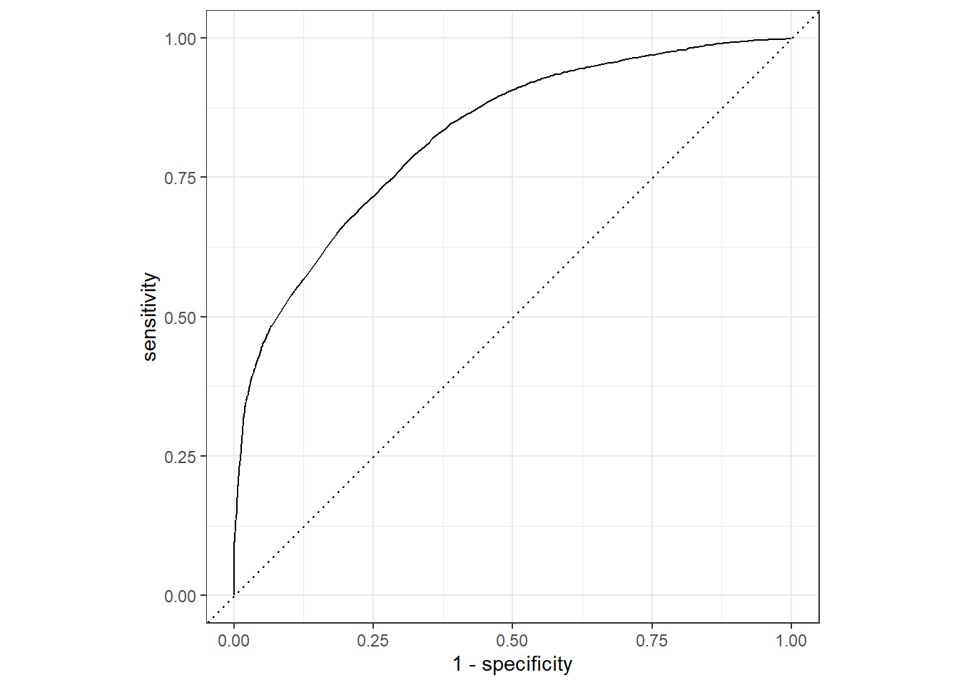
    roc_auc(pred_df, truth = !!sym(truth_col), .pred_1)
  ) %>%
    map_df(bind_rows) %>%
    select(.metric, .estimate) %>%
    pivot_wider(names_from = .metric, values_from = .estimate) %>%
    mutate(Model = model_name)
}

# Combine all model results
all_results <- bind_rows(
  get_metrics(test_pred_tet, "Tetracycline", "Tetracycline"),
  get_metrics(test_pred_ami, "Aminoglycoside", "Aminoglycoside"),
  get_metrics(test_pred_sul, "Sulfonamide", "Sulfonamide"),
  get_metrics(test_pred_bet, "Beta_lactam", "Beta-lactam"),
  get_metrics(test_pred_phe, "Phenicol", "Phenicol"),
  get_metrics(test_pred5, "amr_prevalence", "General AMR")
) %>%
  select(Model, roc_auc, sens, spec, accuracy, precision)

# Create the GT Table
all_results %>%
  gt() %>%
  tab_header(
    title = "Random Forest Model Performance",
    subtitle = "Predicting AMR Classes from Metadata"
  ) %>%
  fmt_number(columns = 2:6, decimals = 3) %>%
  cols_label(
    Model = "Resistance Class",
    roc_auc = "ROC AUC",
    sens = "Sensitivity",
    spec = "Specificity",
    accuracy = "Accuracy",
    precision = "Precision"
  ) %>%
  data_color(columns = roc_auc, palette = "Blues") %>%
  gtsave(here("results/tables/amr_model_performance.html"))  

Publication ready tables and figures

library(vip)
library(ggplot2)
library(here)

# 1. Corrected VIP Plot
amr_vip_pub <- rf_fit_amr %>%
  extract_fit_engine() %>%
  # Use vi_get_variable_importance to pull the permutation scores already calculated by ranger
  vi() %>% 
  mutate(Variable = case_when(
    Variable == "top_20" ~ "Serovar (Top 20)",
    Variable == "Source.type" ~ "Isolation Source",
    Variable == "sample_month" ~ "Month of Collection",
    TRUE ~ Variable
  )) %>%
  ggplot(aes(x = reorder(Variable, Importance), y = Importance)) +
  geom_col(fill = "steelblue", width = 0.7) +
  coord_flip() +
  theme_bw() +
  labs(
    title = "Predictive Power of Metadata Features",
    subtitle = "Random Forest: General AMR Prevalence",
    x = NULL,
    y = "Importance (Permutation Importance)"
  ) +
  theme(plot.title = element_text(face = "bold"))

# Save with publication specs
ggsave(here("results/figures/amr_vip_publication.png"), amr_vip_pub, dpi = 300, width = 7, height = 4)

# 2. ROC Curve Plot (Remains the same, just ensured amr_roc_pub is assigned)
amr_roc_pub <- test_pred5 %>%
  roc_curve(truth = amr_prevalence, .pred_1) %>%
  ggplot(aes(x = 1 - specificity, y = sensitivity)) +
  geom_path(color = "darkred", linewidth = 1) +
  geom_abline(lty = 3, color = "gray50") + 
  annotate("text", x = 0.75, y = 0.25, label = "AUC = 0.825", size = 5, fontface = "bold") +
  theme_bw() +
  coord_equal() +
  labs(
    title = "ROC Curve: General AMR Classification",
    x = "1 - Specificity (False Positive Rate)",
    y = "Sensitivity (True Positive Rate)"
  )

ggsave(here("results/figures/amr_roc_publication.png"), amr_roc_pub, dpi = 300, width = 6, height = 6)

# 3. Probability Density Plot
amr_density_pub <- ggplot(test_pred5, aes(x = .pred_1, fill = amr_prevalence)) +
  geom_density(alpha = 0.6, color = "white") +
  scale_fill_manual(values = c("#D55E00", "#56B4E9"), 
                    labels = c("Resistant", "Susceptible"),
                    name = "Observed Status") +
  theme_bw() +
  labs(
    title = "Predicted Probability Distribution",
    subtitle = "Separation of Resistant vs. Susceptible Classes",
    x = "Predicted Probability of Resistance",
    y = "Density"
  ) +
  theme(legend.position = "bottom")

ggsave(here("results/figures/amr_density_publication.png"), amr_density_pub, dpi = 300, width = 7, height = 5)